Dimensionality Reduction: Latent Variable Modelling

ML Foundations Course Notebook Setup

Review

Clustering

Clustering

• Common approach for grouping data points
• Assigns data points to discrete groups
• Examples include:
  • Animal classification
  • Political affiliation grouping

Clustering vs Vector Quantisation

• Clustering expects gaps between groups in data density
• Vector quantization may not require density gaps
• For practical purposes, both involve:
  • Allocating points to groups
  • Determining optimal number of groups

\(k\)-means Clustering

• Simple iterative clustering algorithm
• Key steps:
  1. Initialize with random centers
  2. Assign points to nearest center
  3. Update centers as cluster means
  4. Repeat until stable

Objective Function

• Minimizes sum of squared distances: \[ E=\sum_{j=1}^K \sum_{i\ \text{allocated to}\ j} \left(\mathbf{ y}_{i, :} - \boldsymbol{ \mu}_{j, :}\right)^\top\left(\mathbf{ y}_{i, :} - \boldsymbol{ \mu}_{j, :}\right) \]
• Solution not guaranteed to be global or unique
• Represents a non-convex optimization problem

Task

• Task: associate data points with different labels.
• Labels are not provided by humans.
• Process is intuitive for humans - we do it naturally.

Platonic Ideals

• Greek philosopher Plato considered the concept of ideals
• The Platonic ideal bird is the most bird-like bird
• In clustering, we find these ideals as cluster centers
• Data points are allocated to their nearest center

Mathematical Formulation

• Represent objects as data vectors \(\mathbf{ x}_i\)
• Represent cluster centers as vectors \(\boldsymbol{ \mu}_j\)
• Define similarity/distance between objects and centers
• Distance function: \(d_{ij} = f(\mathbf{ x}_i, \boldsymbol{ \mu}_j)\)

Squared Distance

• Common choice: squared distance \[ d_{ij} = (\mathbf{ x}_i - \boldsymbol{ \mu}_j)^2 \]
• Goal: find centers close to many data points

Objective Function

• Given similarity measure, need number of cluster centers, \(K\).
• Find their location by allocating each center to a sub-set of the points and minimizing the sum of the squared errors, \[ E(\mathbf{M}) = \sum_{i \in \mathbf{i}_j} (\mathbf{ x}_i - \boldsymbol{ \mu}_j)^2 \] here \(\mathbf{i}_j\) is all indices of data points allocated to the \(j\)th center.

\(k\)-Means Clustering

• \(k\)-means clustering is simple and quick to implement.
• Very initialisation sensitive.

Initialisation

• Initialisation is the process of selecting a starting set of parameters.
• Optimisation result can depend on the starting point.
• For \(k\)-means clustering you need to choose an initial set of centers.
• Optimisation surface has many local optima, algorithm gets stuck in ones near initialisation.

\(k\)-Means Clustering

❮ ❯

Clustering with the \(k\)-means clustering algorithm.

\(k\)-Means Clustering

\(k\)-means clustering by Alex Ihler

Hierarchical Clustering

• Form taxonomies of the cluster centers
• Like humans apply to animals, to form phylogenies
• Builds a tree structure showing relationships between data points
• Two main approaches:
  • Agglomerative (bottom-up): Start with individual points and merge
  • Divisive (top-down): Start with one cluster and split

Oil Flow Data

Phylogenetic Trees

• Hierarchical clustering of genetic sequence data
• Creates evolutionary trees showing species relationships
• Estimates common ancestors and mutation timelines
• Critical for tracking viral evolution and outbreaks

Product Clustering

• Hierarchical clustering for e-commerce products
• Creates product taxonomy trees
• Splits into nested categories (e.g. Electronics → Phones → Smartphones)

Hierarchical Clustering Challenge

• Many products belong in multiple clusters (e.g. running shoes are both ‘sporting goods’ and ‘clothing’)
• Tree structures are too rigid for natural categorization
• Human concept learning is more flexible:
  • Forms overlapping categories
  • Learns abstract rules
  • Builds causal theories

Other Clustering Approaches

• Spectral clustering: Graph-based non-convex clustering
• Dirichlet process: Infinite, non-parametric clustering

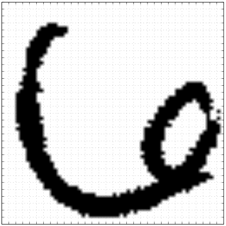
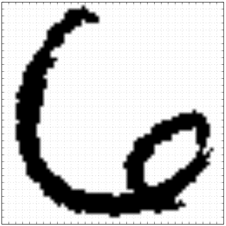
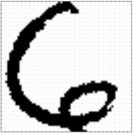
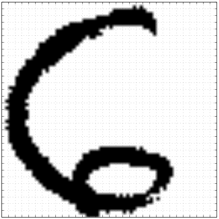
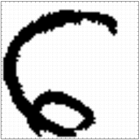
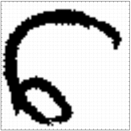
High Dimensional Data

• USPS Data Set Handwritten Digit
• 3648 dimensions (64 rows, 57 columns)
• Space contains much more than just this digit.

USPS Samples

❮ ❯

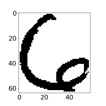
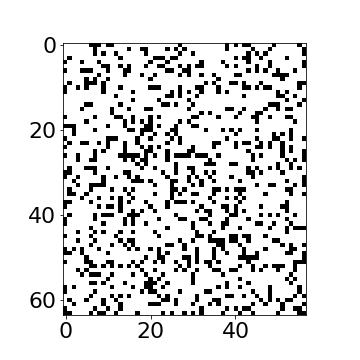
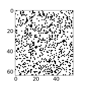
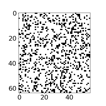
• Even if we sample every nanonsecond from now until end of universe you won’t see original six!

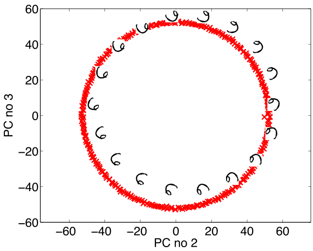
Simple Model of Digit

• Rotate a prototype

❮ ❯

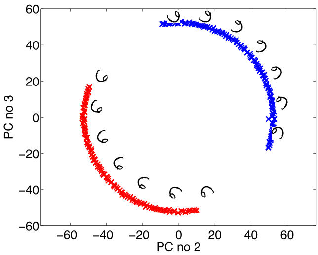
Low Dimensional Manifolds

• Pure rotation is too simple
  • In practice data may undergo several distortions.
• For high dimensional data with structure:
  • We expect fewer distortions than dimensions;
  • Therefore we expect the data to live on a lower dimensional manifold.
  • Conclusion: Deal with high dimensional data by looking for a lower dimensional non-linear embedding.

High Dimensional Data Effects

• High dimensional spaces behave very differently from our 3D intuitions
• Two key effects:
  • Data moves to a “shell” at one standard deviation from mean
  • Distances between points become constant
• Let’s see this experimentally

Pairwise Distances in High-D Gaussian Data

Pairwise Distances in High-D Gaussian Data

• Plot shows pairwise distances in high-D Gaussian data
• Red line: theoretical gamma distribution
• Notice tight concentration of distances

Structured High Dimensional Data

• What about data with underlying structure?
• Let’s create data that lies on a 2D manifold
• Embed it in 1000D space

Pairwise Distances in Structured High-D Data

Pairwise Distances in Structured High-D Data

• Distance distribution differs from pure high-D case
• Matches 2D theoretical curve better than 1000D
• Real data often has low intrinsic dimensionality
• This is why PCA and other dimension reduction works!

High Dimensional Effects in Real Data

Oil Flow Data

Implications for Dimensionality Reduction

Latent Variables and Dimensionality Reduction

• Real data often has lower intrinsic dimensionality than measurements
• Examples:
  • Motion capture: Many coordinates but few degrees of freedom
  • Genetic data: Thousands of genes controlled by few regulators
  • Images: Millions of pixels but simpler underlying structure

Latent Variable Example

Latent Variable Example

• Example shows 2D data described by 1D latent variable
• Left: Data in original 2D space
• Right: Same data represented by single latent variable \(z\)
• Goal: Find these simpler underlying representations

Latent Variables

Your Personality

Factor Analysis Model

\[ \mathbf{ y}= \mathbf{f}(\mathbf{ z}) + \boldsymbol{ \epsilon}, \]

\[ \mathbf{f}(\mathbf{ z}) = \mathbf{W}\mathbf{ z} \]

Closely Related to Linear Regression

\[ \mathbf{f}(\mathbf{ z}) = \begin{bmatrix} f_1(\mathbf{ z}) \\ f_2(\mathbf{ z}) \\ \vdots \\ f_p(\mathbf{ z})\end{bmatrix} \]

\[ f_j(\mathbf{ z}) = \mathbf{ w}_{j, :}^\top \mathbf{ z}, \]

\[ \epsilon_j \sim \mathscr{N}\left(0,\sigma^2_j\right). \]

Data Representation

\[ \mathbf{Y} = \begin{bmatrix} \mathbf{ y}_{1, :}^\top \\ \mathbf{ y}_{2, :}^\top \\ \vdots \\ \mathbf{ y}_{n, :}^\top\end{bmatrix}, \]

\[ \mathbf{F} = \mathbf{Z}\mathbf{W}^\top, \]

Latent Variables vs Linear Regression

\[ x_{i,j} \sim \mathscr{N}\left(0,1\right), \] and we can write the density governing the latent variable associated with a single point as, \[ \mathbf{ z}_{i, :} \sim \mathscr{N}\left(\mathbf{0},\mathbf{I}\right). \]

\[ \mathbf{f}_{i, :} = \mathbf{f}(\mathbf{ z}_{i, :}) = \mathbf{W}\mathbf{ z}_{i, :} \]

\[ \mathbf{f}_{i, :} \sim \mathscr{N}\left(\mathbf{0},\mathbf{W}\mathbf{W}^\top\right) \]

Data Distribution

\[ \mathbf{ y}_{i, :} = \sim \mathscr{N}\left(\mathbf{0},\mathbf{W}\mathbf{W}^\top + \boldsymbol{\Sigma}\right) \]

\[ \boldsymbol{\Sigma} = \begin{bmatrix}\sigma^2_{1} & 0 & 0 & 0\\ 0 & \sigma^2_{2} & 0 & 0\\ 0 & 0 & \ddots & 0\\ 0 & 0 & 0 & \sigma^2_p\end{bmatrix}. \]

Mean Vector

\[ \mathbf{ y}_{i, :} = \mathbf{W}\mathbf{ z}_{i, :} + \boldsymbol{ \mu}+ \boldsymbol{ \epsilon}_{i, :} \]

\[ \boldsymbol{ \mu}= \frac{1}{n} \sum_{i=1}^n \mathbf{ y}_{i, :}, \] \(\mathbf{C}= \mathbf{W}\mathbf{W}^\top + \boldsymbol{\Sigma}\)

Principal Component Analysis

Hotelling (1933) took \(\sigma^2_i \rightarrow 0\) so \[ \mathbf{ y}_{i, :} \sim \lim_{\sigma^2 \rightarrow 0} \mathscr{N}\left(\mathbf{0},\mathbf{W}\mathbf{W}^\top + \sigma^2 \mathbf{I}\right). \]

Degenerate Covariance

\[ p(\mathbf{ y}_{i, :}|\mathbf{W}) = \lim_{\sigma^2 \rightarrow 0} \frac{1}{(2\pi)^\frac{p}{2} |\mathbf{W}\mathbf{W}^\top + \sigma^2 \mathbf{I}|^{\frac{1}{2}}} \exp\left(-\frac{1}{2}\mathbf{ y}_{i, :}\left[\mathbf{W}\mathbf{W}^\top+ \sigma^2 \mathbf{I}\right]^{-1}\mathbf{ y}_{i, :}\right), \]

Computation of the Marginal Likelihood

\[ \mathbf{ y}_{i,:}=\mathbf{W}\mathbf{ z}_{i,:}+\boldsymbol{ \epsilon}_{i,:},\quad \mathbf{ z}_{i,:} \sim \mathscr{N}\left(\mathbf{0},\mathbf{I}\right), \quad \boldsymbol{ \epsilon}_{i,:} \sim \mathscr{N}\left(\mathbf{0},\sigma^{2}\mathbf{I}\right) \]

\[ \mathbf{W}\mathbf{ z}_{i,:} \sim \mathscr{N}\left(\mathbf{0},\mathbf{W}\mathbf{W}^\top\right) \]

\[ \mathbf{W}\mathbf{ z}_{i, :} + \boldsymbol{ \epsilon}_{i, :} \sim \mathscr{N}\left(\mathbf{0},\mathbf{W}\mathbf{W}^\top + \sigma^2 \mathbf{I}\right) \]

Linear Latent Variable Model II

Probabilistic PCA Max. Likelihood Soln (Tipping and Bishop (1999))

\[p\left(\mathbf{Y}|\mathbf{W}\right)=\prod_{i=1}^{n}\mathscr{N}\left(\mathbf{ y}_{i, :}|\mathbf{0},\mathbf{W}\mathbf{W}^{\top}+\sigma^{2}\mathbf{I}\right)\]

Linear Latent Variable Model II

Probabilistic PCA Max. Likelihood Soln (Tipping and Bishop (1999)) \[ p\left(\mathbf{Y}|\mathbf{W}\right)=\prod_{i=1}^{n}\mathscr{N}\left(\mathbf{ y}_{i,:}|\mathbf{0},\mathbf{C}\right),\quad \mathbf{C}=\mathbf{W}\mathbf{W}^{\top}+\sigma^{2}\mathbf{I} \] \[ \log p\left(\mathbf{Y}|\mathbf{W}\right)=-\frac{n}{2}\log\left|\mathbf{C}\right|-\frac{1}{2}\text{tr}\left(\mathbf{C}^{-1}\mathbf{Y}^{\top}\mathbf{Y}\right)+\text{const.} \] If \(\mathbf{U}_{q}\) are first \(q\) principal eigenvectors of \(n^{-1}\mathbf{Y}^{\top}\mathbf{Y}\) and the corresponding eigenvalues are \(\boldsymbol{\Lambda}_{q}\), \[ \mathbf{W}=\mathbf{U}_{q}\mathbf{L}\mathbf{R}^{\top},\quad\mathbf{L}=\left(\boldsymbol{\Lambda}_{q}-\sigma^{2}\mathbf{I}\right)^{\frac{1}{2}} \] where \(\mathbf{R}\) is an arbitrary rotation matrix.

Practical Considerations

When Dimensionality Reduction Fails

• Dimensionality reduction can fail in several key scenarios:
  • Truly high dimensional data with no simpler structure
  • Highly nonlinear relationships between dimensions
  • Varying intrinsic dimensionality across data

The Swiss Roll Example

• Classic example of nonlinear structure
• 2D manifold embedded in 3D
• Linear methods like PCA fail
• Requires nonlinear methods (t-SNE, UMAP)

Common Failure Modes

• Key failure scenarios:
  • Linear methods on nonlinear manifolds
  • Assuming global structure when only local exists
  • Not accounting for noise

f

Principal Component Analysis

• PCA (Hotelling (1933)) is a linear embedding
• Today its presented as:
  • Rotate to find ‘directions’ in data with maximal variance
  • How do we find these directions?

\[ \mathbf{S}=\frac{1}{n}\sum_{i=1}^n\left(\mathbf{ y}_{i, :}-\boldsymbol{ \mu}\right)\left(\mathbf{ y}_{i, :} - \boldsymbol{ \mu}\right)^\top \]

Principal Component Analysis

• Find directions in the data, \(\mathbf{ z}= \mathbf{U}\mathbf{ y}\), for which variance is maximized.

Lagrangian

• Solution is found via constrained optimisation (which uses Lagrange multipliers): \[ L\left(\mathbf{u}_{1},\lambda_{1}\right)=\mathbf{u}_{1}^{\top}\mathbf{S}\mathbf{u}_{1}+\lambda_{1}\left(1-\mathbf{u}_{1}^{\top}\mathbf{u}_{1}\right) \]

• Gradient with respect to \(\mathbf{u}_{1}\) \[\frac{\text{d}L\left(\mathbf{u}_{1},\lambda_{1}\right)}{\text{d}\mathbf{u}_{1}}=2\mathbf{S}\mathbf{u}_{1}-2\lambda_{1}\mathbf{u}_{1}\] rearrange to form \[\mathbf{S}\mathbf{u}_{1}=\lambda_{1}\mathbf{u}_{1}.\] Which is known as an eigenvalue problem.

• Further directions that are orthogonal to the first can also be shown to be eigenvectors of the covariance.

PCA directions

❮ ❯

Maximum variance directions are eigenvectors of the covariance matrix

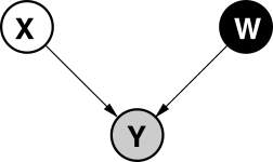
Probabilistic PCA

• Represent data, \(\mathbf{Y}\), with a lower dimensional set of latent variables \(\mathbf{Z}\).

• Assume a linear relationship of the form \[ \mathbf{ y}_{i,:}=\mathbf{W}\mathbf{ z}_{i,:}+\boldsymbol{ \epsilon}_{i,:}, \] where \[ \boldsymbol{ \epsilon}_{i,:} \sim \mathscr{N}\left(\mathbf{0},\sigma^2\mathbf{I}\right) \]

• PPCA defines a probabilistic model where:

  • Data is generated from latent variables through linear transformation
  • Gaussian noise is added to the transformed variables
  • Latent variables have standard Gaussian prior

• Maximum likelihood recovers classical PCA

Graphical model representing probabilistic PCA

Probabilistic PCA

\[ \boldsymbol{\Sigma} = \sigma^2 \mathbf{I}. \]

\[ p(\mathbf{Y}|\mathbf{W}, \sigma^2) = \prod_{i=1}^n\mathscr{N}\left(\mathbf{ y}_{i, :}|\mathbf{0},\mathbf{W}\mathbf{W}^\top + \sigma^2 \mathbf{I}\right) \]

\[ \mathbf{W}= \mathbf{U}\mathbf{L} \mathbf{R}^\top \]

\[ \mathbf{S} = \sum_{i=1}^n(\mathbf{ y}_{i, :} - \boldsymbol{ \mu})(\mathbf{ y}_{i,:} - \boldsymbol{ \mu})^\top, \]

\[ \ell_i = \sqrt{\lambda_i - \sigma^2} \]

PPCA as Manifold Learning

Posterior for Principal Component Analysis

\[ p(\mathbf{ z}_{i, :} | \mathbf{ y}_{i, :}) \]

\[ p(\mathbf{ z}_{i, :} | \mathbf{ y}_{i, :}) \propto p(\mathbf{ y}_{i, :}|\mathbf{W}, \mathbf{ z}_{i, :}, \sigma^2) p(\mathbf{ z}_{i, :}) \]

\[ \log p(\mathbf{ z}_{i, :} | \mathbf{ y}_{i, :}) = \log p(\mathbf{ y}_{i, :}|\mathbf{W}, \mathbf{ z}_{i, :}, \sigma^2) + \log p(\mathbf{ z}_{i, :}) + \text{const} \]

\[ \log p(\mathbf{ z}_{i, :} | \mathbf{ y}_{i, :}) = -\frac{1}{2\sigma^2} (\mathbf{ y}_{i, :} - \mathbf{W}\mathbf{ z}_{i, :})^\top(\mathbf{ y}_{i, :} - \mathbf{W}\mathbf{ z}_{i, :}) - \frac{1}{2} \mathbf{ z}_{i, :}^\top \mathbf{ z}_{i, :} + \text{const} \]

Scikit-learn implementation PCA

Examples: Motion Capture Data

For our first example we’ll consider some motion capture data of a man breaking into a run. Motion capture data involves capturing a 3-d point cloud to represent a character, often by an underlying skeleton. For this data set, from Ohio State University, we have 54 frame of motion capture, each frame containing 102 values, which are the 3-d locations of 34 different points from the subject’s skeleton.

Once the data is loaded in we can examine the first two principal components as follows,

Here because the data is a time course, we have connected points that are neighbouring in time. This highlights the form of the run, which involves 3 paces. This projects in our low dimensional space to 3 loops. We can examin how much residual variance there is in the system by looking at sigma2.

Robot Navigation Example

• Example involving 215 observations of 30 access points.
• Infer location of ‘robot’ and accesspoints.
• This is known as SLAM (simulataneous localization and mapping).

Interpretations of Principal Component Analysis

Relationship to Matrix Factorization

• PCA is closely related to matrix factorisation.

• Instead of \(\mathbf{Z}\), \(\mathbf{W}\)

• Define Users \(\mathbf{U}\) and items \(\mathbf{V}\)

• Matrix factorisation: \[ f_{i, j} = \mathbf{u}_{i, :}^\top \mathbf{v}_{j, :} \] PCA: \[ f_{i, j} = \mathbf{ z}_{i, :}^\top \mathbf{ w}_{j, :} \]

Other Interpretations of PCA: Separating Model and Algorithm

• PCA introduced as latent variable model (a model).
• Solution is through an eigenvalue problem (an algorithm).
• This causes some confusion about what PCA is.

\[ \mathbf{Y}= \mathbf{V} \boldsymbol{\Lambda} \mathbf{U}^\top \]

\[ \mathbf{Y}^\top\mathbf{Y}= \mathbf{U}\boldsymbol{\Lambda}\mathbf{V}^\top\mathbf{V} \boldsymbol{\Lambda} \mathbf{U}^\top = \mathbf{U}\boldsymbol{\Lambda}^2 \mathbf{U}^\top \]

Separating Model and Algorithm

• Separation between model and algorithm is helpful conceptually.
• Even if in practice they conflate (e.g. deep neural networks).
• Sometimes difficult to pull apart.
• Helpful to revisit algorithms with modelling perspective in mind.
  • Probabilistic numerics

PPCA Marginal Likelihood

We have developed the posterior density over the latent variables given the data and the parameters, and due to symmetries in the underlying prediction function, it has a very similar form to its sister density, the posterior of the weights given the data from Bayesian regression. Two key differences are as follows. If we were to do a Bayesian multiple output regression we would find that the marginal likelihood of the data is independent across the features and correlated across the data, \[ p(\mathbf{Y}|\mathbf{Z}) = \prod_{j=1}^p \mathscr{N}\left(\mathbf{ y}_{:, j}|\mathbf{0}, \alpha\mathbf{Z}\mathbf{Z}^\top + \sigma^2 \mathbf{I}\right) \] where \(\mathbf{ y}_{:, j}\) is a column of the data matrix and the independence is across the features, in probabilistic PCA the marginal likelihood has the form, \[ p(\mathbf{Y}|\mathbf{W}) = \prod_{i=1}^n\mathscr{N}\left(\mathbf{ y}_{i, :}|\mathbf{0},\mathbf{W}\mathbf{W}^\top + \sigma^2 \mathbf{I}\right) \] where \(\mathbf{ y}_{i, :}\) is a row of the data matrix \(\mathbf{Y}\) and the independence is across the data points.

Computation of the Log Likelihood

The quality of the model can be assessed using the log likelihood of this Gaussian form. \[ \log p(\mathbf{Y}|\mathbf{W}) = -\frac{n}{2} \log \left| \mathbf{W}\mathbf{W}^\top + \sigma^2 \mathbf{I}\right| -\frac{1}{2} \sum_{i=1}^n\mathbf{ y}_{i, :}^\top \left(\mathbf{W}\mathbf{W}^\top + \sigma^2 \mathbf{I}\right)^{-1} \mathbf{ y}_{i, :} +\text{const} \] but this can be computed more rapidly by exploiting the low rank form of the covariance covariance, \(\mathbf{C}= \mathbf{W}\mathbf{W}^\top + \sigma^2 \mathbf{I}\) and the fact that \(\mathbf{W}= \mathbf{U}\mathbf{L}\mathbf{R}^\top\). Specifically, we first use the decomposition of \(\mathbf{W}\) to write: \[ -\frac{n}{2} \log \left| \mathbf{W}\mathbf{W}^\top + \sigma^2 \mathbf{I}\right| = -\frac{n}{2} \sum_{i=1}^q \log (\ell_i^2 + \sigma^2) - \frac{n(p-q)}{2}\log \sigma^2, \] where \(\ell_i\) is the \(i\)th diagonal element of \(\mathbf{L}\). Next, we use the Woodbury matrix identity which allows us to write the inverse as a quantity which contains another inverse in a smaller matrix: \[ (\sigma^2 \mathbf{I}+ \mathbf{W}\mathbf{W}^\top)^{-1} = \sigma^{-2}\mathbf{I}-\sigma^{-4}\mathbf{W}{\underbrace{(\mathbf{I}+\sigma^{-2}\mathbf{W}^\top\mathbf{W})}_{\mathbf{C}_x}}^{-1}\mathbf{W}^\top \] So, it turns out that the original inversion of the \(p \times p\) matrix can be done by forming a quantity which contains the inversion of a \(q \times q\) matrix which, moreover, turns out to be the quantity \(\mathbf{C}_x\) of the posterior.

Now, we put everything together to obtain: \[ \log p(\mathbf{Y}|\mathbf{W}) = -\frac{n}{2} \sum_{i=1}^q \log (\ell_i^2 + \sigma^2) - \frac{n(p-q)}{2}\log \sigma^2 - \frac{1}{2} \text{tr}\left(\mathbf{Y}^\top \left( \sigma^{-2}\mathbf{I}-\sigma^{-4}\mathbf{W}\mathbf{C}_x \mathbf{W}^\top \right) \mathbf{Y}\right) + \text{const}, \] where we used the fact that a scalar sum can be written as \(\sum_{i=1}^n\mathbf{ y}_{i,:}^\top \mathbf{K}\mathbf{ y}_{i,:} = \text{tr}\left(\mathbf{Y}^\top \mathbf{K}\mathbf{Y}\right)\), for any matrix \(\mathbf{K}\) of appropriate dimensions. We now use the properties of the trace \(\text{tr}\left(\mathbf{A}+\mathbf{B}\right)=\text{tr}\left(\mathbf{A}\right)+\text{tr}\left(\mathbf{B}\right)\) and \(\text{tr}\left(c \mathbf{A}\right) = c \text{tr}\left(\mathbf{A}\right)\), where \(c\) is a scalar and \(\mathbf{A},\mathbf{B}\) matrices of compatible sizes. Therefore, the final log likelihood takes the form: \[ \log p(\mathbf{Y}|\mathbf{W}) = -\frac{n}{2} \sum_{i=1}^q \log (\ell_i^2 + \sigma^2) - \frac{n(p-q)}{2}\log \sigma^2 - \frac{\sigma^{-2}}{2} \text{tr}\left(\mathbf{Y}^\top \mathbf{Y}\right) +\frac{\sigma^{-4}}{2} \text{tr}\left(\mathbf{B}\mathbf{C}_x\mathbf{B}^\top\right) + \text{const} \] where we also defined \(\mathbf{B}=\mathbf{Y}^\top\mathbf{W}\). Finally, notice that \(\text{tr}\left(\mathbf{Y}\mathbf{Y}^\top\right)=\text{tr}\left(\mathbf{Y}^\top\mathbf{Y}\right)\) can be computed faster as the sum of all the elements of \(\mathbf{Y}\circ\mathbf{Y}\), where \(\circ\) denotes the element-wise (or Hadamard) product.

Summary and Key Points