Abstract

In this lab session we will explore dataset joining techniques, implement the Access-Assess-Address framework in practice, work with the DSAIL Porini camera trap data, and build predictive models for animal sightings.

Code Reuse with Fynesse

{We will be reusing some of the functions we created in the first practical. This demonstrates one of the key principles of data science: building reusable code libraries that can be applied across multiple projects.

%%capture
%pip install osmnx

Exercise 1

Install your Fyness library, and run code to show its available.

# Example: Plot a city map using your reusable function
# fynesse.access.plot_city_map('Nyeri, Kenya', -0.4371, 36.9580, 2)

DSAIL-Porini Dataset

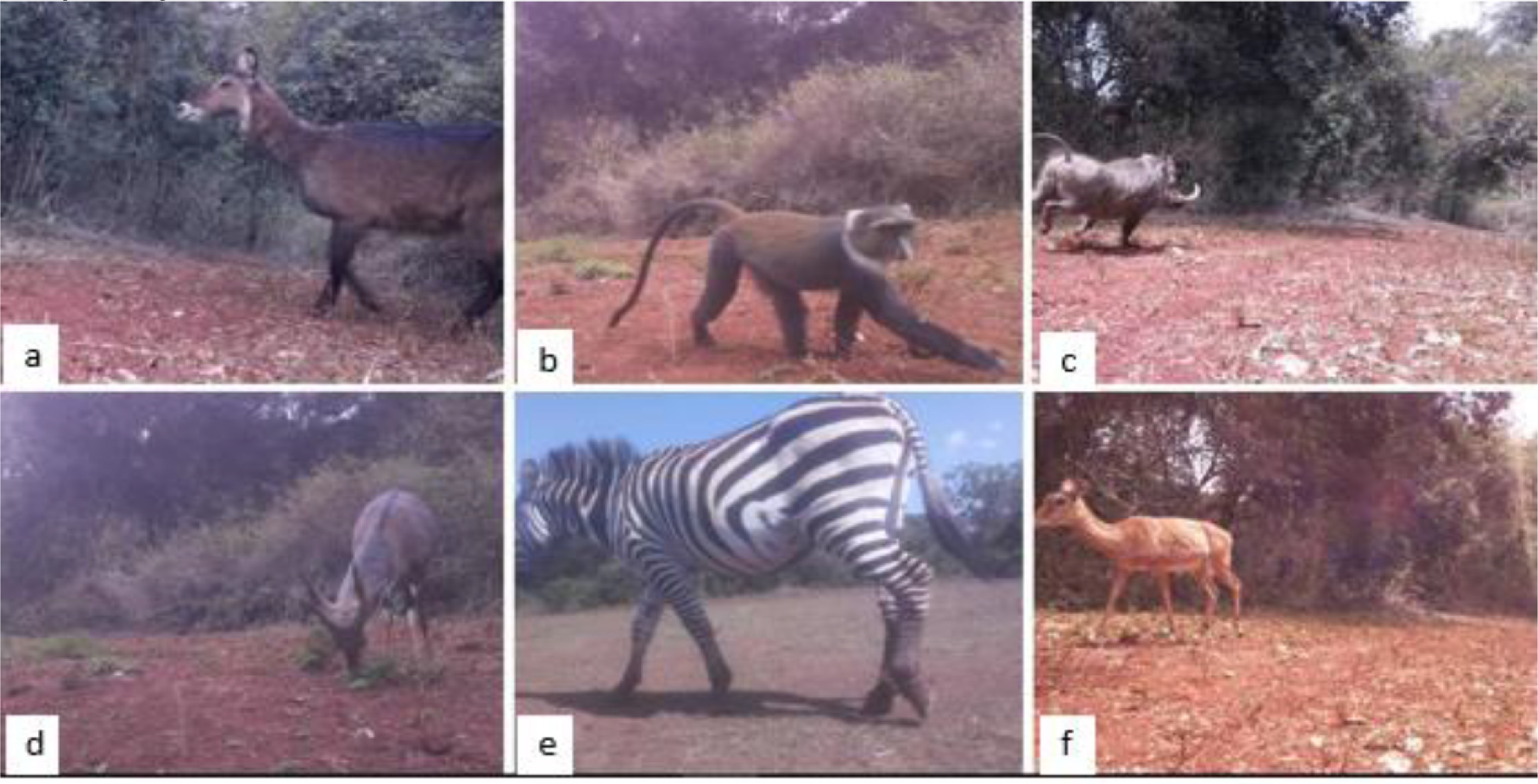
Head over to https://data.mendeley.com/datasets/6mhrhn7rxc/6 to explore the DSAIL-Porini dataset. This dataset contains camera trap images and annotations from Kenya, providing rich information about wildlife patterns and behavior.

Locate the camera_trap_dataset_annotation.xlsx file and make it available in this notebook.

import os
import requests
import pandas as pd

def download_if_not_exists(url, filepath):
    """Download file if it doesn't exist locally"""
    if os.path.exists(filepath):
        print(f"File already exists: {filepath}")
    else:
        print(f"Downloading: {url}")
        response = requests.get(url, stream=True)
        response.raise_for_status()
        with open(filepath, "wb") as f:
            for chunk in response.iter_content(chunk_size=8192):
                f.write(chunk)
        print(f"Downloaded to: {filepath}")
    return filepath

# Download the DSAIL-Porini dataset
porini_file = download_if_not_exists(
    'https://data.mendeley.com/public-files/datasets/6mhrhn7rxc/files/641e83c9-16a3-485c-b247-b5701f8a5540/file_downloaded', 
    'camera_trap_dataset_annotation.xlsx'
)

porini_df = pd.read_excel(porini_file)
porini_df.head()

Joining Datasets

Exercise 2

Geospatial data is particularly useful because it is the most common index in the world, over which so many datasets can be joined. Find the coordinate information in the dataset, and plot it on top of an OSM map.

You may want to deduplicate the coordinates before you plot!

Sighting Predictions

We will use the dataset to create a simple prediction model for the likelihood of animal sightings.

Let’s follow a minimal example of the Access-Assess-Address framework!

Reminder about Neil’s article on the framework here.

Access

Access is already done, partly years ago by the DSAIL team, and two cells above by us. Example tasks within access would be:

• Setting up the cameras in the woods (done)
• Collecting the pictures (done)
• Labeling the dataset (done)
• Making the excel file online accessible (done)
• Downloading the file (done just now)}

porini_df.head()

Assess

Have a look at the dataset for any issues that could stop us from being able to cleanly analyse it.

Some issues:

• Timestamps not readilly available. Hidden in image filenames.
• No timestamps available for one of the cameras.
• No Camera ID, but can be deduced from coordinates.

Decide how it would be best to address these and potentially other issues with the data.

We would like an output dataframe that has a column for counts each animal was spotted by each camera, and rows for each day in the available range. You might want to use this opportunity to practice Pandas MultiIndex.

import pandas as pd
import numpy as np
import re

# Copy original
df = porini_df.copy()

# Normalize species and parse counts
df["Species"] = df["Species"].astype(str).str.strip()

# Extract timestamp from filename
pat = re.compile(r"(\d{4})-(\d{2})-(\d{2})-(\d{2})-(\d{2})-(\d{2})")
def parse_ts(name):
    m = pat.search(str(name))
    if not m:
        return pd.NaT
    y, M, d, h, m_, s = map(int, m.groups())
    return pd.Timestamp(y, M, d, h, m_, s)

df["timestamp"] = df["Filename"].map(parse_ts)
df["date"] = df["timestamp"].dt.date

# Camera ID from rounded lat/lon
df["Latitude"] = df["Latitude"].round(4)
df["Longitude"] = df["Longitude"].round(4)
coord_key = df["Latitude"].astype(str) + "," + df["Longitude"].astype(str)
codes, _ = pd.factorize(coord_key)
df["camera_id"] = pd.Series(codes).map(lambda i: f"C{int(i)+1:03d}")

# Extract camera coordinates dictionary (rounded)
camera_coords = (
    df.drop_duplicates(subset="camera_id")[["camera_id", "Latitude", "Longitude"]]
      .set_index("camera_id")
      .sort_index()
      .apply(tuple, axis=1)
      .to_dict()
)

# Group and count: number of pictures per species per camera per day
daily = (
    df.dropna(subset=["date"])
      .groupby(["date", "camera_id", "Species"])
      .size()
      .reset_index(name="photo_count")
      .pivot_table(index="date", columns=["camera_id", "Species"], values="photo_count", aggfunc="sum")
      .fillna(0)
      .astype(int)
      .sort_index()
)

# Fill missing dates
if not daily.empty:
    full_idx = pd.date_range(start=daily.index.min(), end=daily.index.max(), freq="D").date
    daily = daily.reindex(full_idx).fillna(0).astype(int)
    daily.index.name = "date"

print(camera_coords)
daily.tail()

Huh, looks like we have some more issues.

• “Impala, Monkey” is not a species - should be counted towards two!
• “Can’t Tell” shouldn’t be a species at all.
• Some columns don’t exist (eg. C011 has no ZEBRA). Let’s just fill them with zeros.

Additionally, there probably weren’t 1577 impalas spotted on Christmas Eve 2021. This is a result of burst shots repetitively capturing the same animal. For now, let’s just treat the data as binary, whether at least one photo was taken on that day.

Exercise 3

Use the cell below to implement the changes discussed above, and potentially additional issues.

Statistical Analysis of Sighting Patterns

Exercise 4

Now let’s create a simple prediction system for whether a specific camera captured a species on a given date. Let’s use the whole dataset, except for the prediction target date.

Before we jump into addressing the question, let’s further assess the data. Calculate and plot average probabilities for dates, species, and cameras. You may want to implement some smoothing over dates, or group them into longer ranges.

Extension: which of these relationships that you found are statistically significant?

# TODO

Address: Naive Bayesian Prediction Model

Using the data we collected in the Access stage and understood in Assess, we can now Address our question, and create a naive Bayesian classification model for predicting the probability of a camera sighting a species on a given day.

\[ P(1 \mid c, s, d) = \frac{P(1, c, s, d)}{P(c, s, d)} \]

\[ \text{Using chain rule:} \quad P(1, c, s, d) = P(1) \cdot P(c, s, d \mid 1) \]

\[ \text{Using conditional independence:} \quad P(c, s, d \mid 1) = P(c \mid 1) \cdot P(s \mid 1) \cdot P(d \mid 1) \]

\[ P(1 \mid c, s, d) = \frac{P(1) \cdot P(c \mid 1) \cdot P(s \mid 1) \cdot P(d \mid 1)}{P(c,s,d)} \]

\[ \text{Using Bayes' rule:} \quad P(c \mid 1) = \frac{P(1 \mid c) \cdot P(c)}{P(1)} \quad \text{(and similarly for $s$ and $d$)} \]

\[ \Rightarrow P(1 \mid c, s, d) = \frac{P(1) \cdot \frac{P(1 \mid c) \cdot P(c)}{P(1)} \cdot \frac{P(1 \mid s) \cdot P(s)}{P(1)} \cdot \frac{P(1 \mid d) \cdot P(d)}{P(1)}}{P(c,s,d)} \]

\[ = \frac{P(1 \mid c) \cdot P(1 \mid s) \cdot P(1 \mid d) \cdot P(c) \cdot P(s) \cdot P(d)}{P(1)^2 \cdot P(c,s,d)} \]

\[ \text{Assuming independence:} \]

\[ P(1 \mid c,s,d)=\frac{P(1 \mid c) \cdot P(1 \mid s) \cdot P(1 \mid d)}{P(1)^2} \]

\[ \begin{align*} &c = \text{camera ID (e.g., C001)} \\ &s = \text{species (e.g., IMPALA)} \\ &d = \text{smoothed date (e.g., month, or Gaussian-filtered day)} \end{align*} \]

Exercise 5

Implement the model below.

Well done! We should now have a working Access-Assess-Address data science pipeline! Let’s see how it does.

#

Evaluation

The data is extremely sparse, with less than 1% of values being 1. This is a challenge, as checking naive accuracy would make always-zero a very very good predictor.

Let’s evaluate our prediction system using log-loss i.e. cross-entropy:

\[ \mathcal{L} = - \frac{1}{N} \sum_{i=1}^{N} \Big[ y_i \, \log(\hat{p}_i) + (1 - y_i) \, \log(1 - \hat{p}_i) \Big] \]

Exercise 6

Implement the loss function below.

For reference, predicting a constant probability (eg. 0.5%) gives a loss of around 0.026. This should be the benchmark number we want to improve on. If your model does better than that, well done!

Note: our approach included look-ahead bias - making predictions based on data that we would not have access to at the time. For real-life deployment, we would need to limit our training data to before individual test cases.

Improving the Method: Correlated Variables

The model above was quite simplified, and it disregarded any correlations between the three variables. Since cameras are close to each other, maybe they are more likely to capture the same animals on the same day? Maybe some animals like or avoid some areas, or some other animals? If any of the above is true, we can’t really be using simple Bayes’ rule classification.

Exercise 7

Analyse the data again to find the strongest relationships which can be used to improve predictions. Plot correlation matrices and other helpful charts.

Have a short read through the DSAIL-Porini paper for inspiration about other probability analyses that can be done here.

Extension: Use what you found to improve your prediction model, and compare it against the previous one.

from typing import Union
import pandas as pd
import numpy as np
from datetime import date as DateType

def improved_sighting_probability(df, camera, species, date) -> float:
    """
    Removes a specific observation and estimates the probability of sighting
    a given species at a given camera on a specific date.

    Parameters:
        df (pd.DataFrame): DataFrame with MultiIndex columns (camera, species) and datetime.date index.
        camera (str): Camera ID (e.g. 'C001').
        species (str): Species name (e.g. 'IMPALA').
        date (str or datetime.date or pd.Timestamp): Date of the observation.

    Returns:
        float: Estimated sighting probability - TODO.
    """
    if isinstance(date, str) or isinstance(date, pd.Timestamp):
        date = pd.to_datetime(date).date()

    df_blind = df.copy()
    df_blind.loc[date, (camera, species)] = None

    #TODO

    raise NotImplementedError("Prediction logic not implemented yet.")

Extended Exercises

We didn’t use all of the available data when we just classified days as “sighting” or “no sighting.” Extend your analysis to include all the information in the file, like numbers of sightings and numbers of animals in the photos.

This will be quite challenging due to burst shots - assess the dataset and come up with a good definition of what a burst is, and a data structure that has the information you chose as important.

Example burst data: - Camera, Date, Species - Time Start, Time End - Number of photos - Average/most animals in a photo

Particular challenge around deduplicating multi-species sightings.

Exercise 8

Use this additional data and repeat the analysis you did above. Aim to further improve predictions and write a new function like burst_sighting_probability('C001', 'IMPALA', '2021-12-24').

Exercise 9

Compare the results and note the improvement (or lack thereof) against the two previous prediction functions you created.

Exercise 10

What other benefits does your new system provide? Can you modify it to provide more predictions, like the expected number of sightings, the number of animals?

Database Integration with SQLite

Throughout the course you will work with various datasets and data formats. An SQL database is one of the most common ways to store large amounts of data. We recognise that many of you may be familiar with this already, but let’s use this example to build a small toy database of animal sightings based on the excel file and the dataframes we created.

Exercise 11

• Create a local database (eg. sqlite3).
• Add a table with animal sighting data.
• Add a table with camera coordinates data.
• Set indices on columns you might search by (eg. CameraID, Date). Make sure the index types make sense!
• Look into multi column indices, and set one on Latitude and Longitude.
• Demonstrate success with a couple SQL queries, eg. counting IMPALA sightings within a 200m square around -0.3866, 36.9649.

Helpful links:

SQL Intro, Creating Tables, Indices, Joins

Multi-Column Indices

Remember to include reusable code from this and previous exercises in your Fynesse library!

Extended Analysis: Burst Detection

We didn’t use all of the available data when we just classified days as “sighting” or “no sighting.” Change your analysis to include the number of sightings and the number of animals in the photos.

This will be quite challenging due to burst shots - assess the dataset and come up with a good definition of what a burst is, and a data structure that has the information you chose as important.

Example burst data: - Camera, Date, Species - Time Start, Time End - Number of photos - Average/most animals in a photo

Particular hardship around deduplicating multi-species sightings.

Exercise 12

Use this additional data and repeat the analysis you did above. Further improve predictions and write a new function like burst_sighting_probability('C001', 'IMPALA', '2021-12-24').

Exercise 13

Compare the results and note the improvement (or lack thereof) against the two previous prediction functions you created.

Exercise 14

What other benefits does your new system provide? Can you modify it to provide more predictions, like the expected number of sightings, the number of animals?

End of Practical 3

 _______  __   __  _______  __    _  ___   _  _______  __
|       ||  | |  ||   _   ||  |  | ||   | | ||       ||  |
|_     _||  |_|  ||  |_|  ||   |_| ||   |_| ||  _____||  |
  |   |  |       ||       ||       ||      _|| |_____ |  |
  |   |  |       ||       ||  _    ||     |_ |_____  ||__|
  |   |  |   _   ||   _   || | |   ||    _  | _____| | __
  |___|  |__| |__||__| |__||_|  |__||___| |_||_______||__|

References