Practical 2: Data and Python

Abstract

In this lab session we will explore the use of SQL and pandas with a football data base.

Data and Python

The Data

We’ll be using a partial EA FC 25 database for this workshop.

Figure:

Find it in this GitHub repo: radzim/football_data

import os, subprocess

repo_url = "https://github.com/radzim/football_data.git"
repo_dir = "football_data"

if not os.path.exists(repo_dir):
    subprocess.run(["git", "clone", repo_url], check=True)

What we have:

os.listdir('football_data')

with open('football_data/models.csv') as f:
    print(f.read()[:394])

Introduction

If you wish to make an apple pie from scratch, you must first invent the universe. - Carl Sagan

In Python we deal with information all the time. Every variable, every list is data stored and operated on.

text = 'hello world'
year = 2025
primes = [2, 3, 5, 7]

Memory

Something not many people think about, is what these actually are, under the hood.

True, '1', 1, 1.0

Someone coming from a C++ background, would call the above primitives - expecting them to just be raw data in memory.

type(True), type('1'), type(1), type(1.0)

Let’s check this assumption - we would expect a bool to take 1 bit or 1 byte, int 1-4 bytes, string 1-2 bytes, and float 4 bytes

import sys

sys.getsizeof(True), sys.getsizeof('1'), sys.getsizeof(1), sys.getsizeof(1.0)

The above numbers look nothing like our predictions - why is that?

Turns out, in Python, everything is actually an object. The simple 1 we saw above is represented in memory as:

ob_refcnt: 8 bytes
ob_type: 8 bytes
ob_size: 8 bytes (Py_ssize_t)
ob_digit: 4 bytes per 30 bits of int

The four types above are somewhat special in Python too, with a slightly different implementation than other objects. Other types and structures are built up in similar ways, but don’t store actual values inside, but rather pointers to “primitives” objects.

In the example above we needed 28 bytes to encode one bit of information. Native Python is insanely inefficient for operations on large data. This memory design also impacts other ways in which we accelerate data operations, namely caching.

Data Structures

Hardware acceleration and memory layouts can only take us so far, usually some constant multiplier faster. For real step-changes in performance, we need to be mathematically clever about how we arrange our data.

Basic data structures

list
tuple
set
dict

By default, you would use a list for data. But other data types have their advantages too - set has very quick lookups, dict has quick lookups and stores values, and tuple is mutable and hashable (more on that later).

Example where set massively outperforms a list:

import time
import random

data_list = list(range(1000000))
queries = [random.randint(0, 2000000) for _ in range(1000)]

start_time = time.time()
hits = sum(1 for q in queries if q in data_list)
print(hits, time.time() - start_time)

data_set = set(range(1000000))

start_time = time.time()
hits = sum(1 for q in queries if q in data_set)
print(hits, time.time() - start_time)

Other useful data structures

Counter

from collections import Counter

with open('football_data/leagueteamlinks.csv') as f:
  leagues = ([x.split(',')[12] for x in f.read().split('\n')[1:-1]]) # 13th column is leagueid
c = Counter(leagues)
print(c)

To be expanded as I get reminded of cool things.

Mutability

l1, l2, l3 = ['apple'], ['banana'], ['cherry']
list_of_lists = [l1, l2, l3]
s1, s2, s3 = 'apple', 'banana', 'cherry'
list_of_strings = [s1, s2, s3]
print(list_of_lists, list_of_strings)

l3[0] = 'cranberry'
s3 = 'cranberry'
print(l3, s3)
print(list_of_lists)
print(list_of_strings)

This will be particularly important when working with Pandas, when operations on rows will sometimes be in-place, and sometimes return new objects. You will get serious silent bugs if you’re not careful.

Hashability

Python property, means roughly “can convert this to a number for lookups.”

try:
    s = {'a', 'b', 'c', ['d', 'e']}
    print(s)
except TypeError as e:
    print(e)

{'a', 'b', 'c', ('d', 'e')}

dict_ = {1: 'one', 2: 'two', (3, 4): 'three or four'}
dict_[(3, 4)]

Spatial (and Temporal) locality

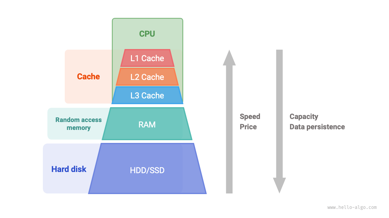
Figure:

Spatial locality means a program is likely to access nearby memory addresses soon after accessing one (e.g., iterating through an array). CPUs exploit both by loading data from RAM based on expected patterns of use.

Temporal locality benefits from keeping recently used data in cache, while spatial locality benefits from prefetching adjacent data to speed up sequential access.

Let’s test it out using a toy example - summing over 1m numbers, first in order, then randomly.

import time

arr = [1]*10000000
indices = list(range(10000000))
start_time = time.time()
s = 0
for i in indices:
    s += arr[i]
print(s, time.time()-start_time)

import random

arr = [1]*10000000
indices = list(range(10000000))
random.shuffle(indices)
start_time = time.time()
s = 0
for i in indices:
    s += arr[i]
print(s, time.time()-start_time)

Mathematically speaking, these two operations are the same. Yet one takes about 5-10 times longer. This is exactly due to locality - it’s much faster to read data that’s right next to each other in memory.

Python’s huge representations of data, and overused pointers, limit the capabilities of caching.

It is a little bit silly to be optimising Python code, given how much inefficiency our choice of language brings on, but the considerations are still important, and translate to other systems you may build.

# temporal locality would be this - difference is quite small
# import time
# arr = [1]*10000000
# indices = [1]*10000000
# start_time = time.time()
# s = 0
# for i in indices:
#     s += arr[i]
# print(s, time.time()-start_time)

Numerical Computation np

import numpy as np

Probably all of you have written the above line hundreds of times. Let’s recap why we do it.

NumPy is a Python library for fast numerical computing. It’s the foundation for many data science and machine learning libraries, including Pandas. Under the hood, NumPy is written largely in C to achieve high performance.

arr = [1]*10000000
indices = list(range(10000000))
start_time = time.time()
s = 0
for i in indices:
    s += arr[i]
print(s, time.time()-start_time)

np_arr = np.array(arr)
start_time = time.time()
s = np_arr.sum()
print(s, time.time()-start_time)

NumPy is insanely fast. Use it everywhere you can!

Cheat Sheet

Create Arrays

a = np.array([1, 2, 3, 4, 5])
print(a)        # [1 2 3 4 5]
print(a.shape)  # (5,)

Multidimensional array:

b = np.array([[1, 2, 3],
              [4, 5, 6]])
print(b)
# [[1 2 3]
#  [4 5 6]]
print(b.shape)  # (2, 3)

Array Slicing

arr = np.array([10, 20, 30, 40, 50])
print(arr[1:4])   # [20 30 40]
print(arr[:3])    # [10 20 30]
print(arr[-2:])   # [40 50]

2D slicing:

b = np.array([[1, 2, 3],
              [4, 5, 6],
              [7, 8, 9]])
print(b[0:2, 1:3])
# [[2 3]
#  [5 6]]

Fancy Indexing & Boolean Masking

arr = np.array([5, 10, 15, 20, 25])
print(arr[[0, 2, 4]])    # [ 5 15 25]
print(arr[arr > 10])     # [15 20 25]

Vectorized Operations

x = np.array([1, 2, 3])
y = np.array([10, 20, 30])

print(x + y)    # [11 22 33]
print(x * y)    # [10 40 90]
print(x ** 2)   # [1 4 9]

Cumulative Sum & Other Reductions

arr = np.array([1, 2, 3, 4])
print(np.cumsum(arr))  # [ 1  3  6 10]
print(np.sum(arr))     # 10
print(np.prod(arr))    # 24
print(np.mean(arr))    # 2.5

Reshaping Arrays

arr = np.arange(1, 13)
reshaped = arr.reshape(3, 4)
print(reshaped)
# [[ 1  2  3  4]
#  [ 5  6  7  8]
#  [ 9 10 11 12]]

Useful Utilities

np.zeros((2, 3))     # [[0. 0. 0.]
                     #  [0. 0. 0.]]
np.ones((2, 3))      # [[1. 1. 1.]
                     #  [1. 1. 1.]]
np.arange(0, 10, 2)  # [0 2 4 6 8]
np.linspace(0, 1, 5) # [0.   0.25 0.5  0.75 1. ]

Structured Data pd

import pandas as pd

Again, probably all of you have written the above line hundreds of times. Let’s recap why we do it.

Pandas is a library built on top of NumPy. It provides two main data structures: Series (1D) and DataFrame (2D) to handle structured data efficiently.

Pandas supports data cleaning, transformation, aggregation, merging, time-series analysis, and visualisation with minimal code. It integrates neatly with common libraries (np, plt, sk, …).

It moves all numerical operations to NumPy, for great speed. It also has builtin support for tonnes of data formats, like csv, xlsx, db … .

One of the most used tools in data science and machine learning.

Cheat Sheet

Create DataFrames

df = pd.DataFrame({
    "playerid": [1, 2, 3, 4],
    "playername": ["Messi", "Ronaldo", "Mbappe", "Haaland"],
    "height": [170, 187, 178, 195]
})
print(df)

Read & Inspect Data

df = pd.read_csv("football_data/players.csv")
print(df.head())      # First 5 rows
print(df.info())      # Column info & types
print(df.describe())  # Stats summary for numeric columns
print(df.columns)     # List of column names
print(df.shape)       # (rows, columns)

Selecting Columns & Rows

df["playername"]                  # Single column - Series
df[["playername", "height"]]      # Multiple columns

df.iloc[0]          # by position
df.loc[0]           # by label
df.iloc[0:3]        # First 3 rows
df.loc[df["height"] > 185]   # Conditional filter

Sorting

df.sort_values("height", ascending=False).head()

Grouping & Aggregation

df.groupby("nationality")["height"].mean()

Merging & Joining

teamplayerlinks = pd.read_csv("football_data/teamplayerlinks.csv")
df_merged = df.merge(teamplayerlinks, on="playerid", how="left")
print(df_merged.head())

Missing Data

df.isna().sum()
df["height"].fillna(df["height"].mean())
df.dropna(subset=["height"])

Explode

df["playername"] = df["playername"].astype(str).str.split(" ")
df = df.explode("playername").reset_index(drop=True)

Exporting Data

df.to_csv("players_clean.csv", index=False)
df.to_pickle("players_clean.pkl")

Avoiding mutability issues

df2 = df.copy()

Apply

df = pd.read_csv('football_data/players.csv')
start = time.time()
df["height_m"] = df["height"].map(lambda x: x / 100)
df["bmi"] = df.apply(lambda x: x["weight"]/x["height_m"]**2, axis=1)
print(time.time()-start)
df["bmi"]
# .map is very similar to `apply` for Series, slightly faster, accepts a dictionary too not just function

Caveat: Apply is not vectorised, not very fast. Use vectorised operations where possible!

df = pd.read_csv('football_data/players.csv')
start = time.time()
df["height_m"] = df["height"]/100
df["bmi"] = df["weight"]/df["height_m"]**2
print(time.time()-start)
df["bmi"]

Pickles

Pickles are a Python way of storing objects as files. Very useful, and usually faster than the naive way of doing things.

t = time.time()
df.to_csv("data.csv")
pd.read_csv("data.csv")
print("csv", time.time() - t)

t = time.time()
df.to_pickle("data.pkl")
pd.read_pickle("data.pkl")
print("pickle", time.time() - t)

Pickle are very general and can store basically any Python object, even functions.

import pickle

def greet(name): return f"Hello, {name}!"
pickle.dump(greet, open("func.pkl", "wb"))
f = pickle.load(open("func.pkl", "rb"))
print(f("World"))

Databases sql

You should already know this from previous courses, but here’s a little recap.

Cheat Sheet

Create Tables & Insert Data

CREATE TABLE players (
    playerid INTEGER PRIMARY KEY,
    playername TEXT,
    height INTEGER
);
INSERT INTO players (playerid, playername, height) VALUES
(1, 'Messi', 170),
(2, 'Ronaldo', 187),
(3, 'Mbappe', 178),
(4, 'Haaland', 195);

Read & Inspect Data

SELECT * FROM players LIMIT 5;
SELECT COUNT(*) FROM players;
PRAGMA table_info(players);
SELECT name FROM sqlite_master WHERE type='table';

Selecting Columns & Rows

SELECT playername FROM players;
SELECT playername, height FROM players;
SELECT * FROM players WHERE playerid = 1;
SELECT * FROM players WHERE height > 185;
SELECT * FROM players LIMIT 3;

Sorting

SELECT * FROM players
ORDER BY height DESC
LIMIT 5;

Grouping & Aggregation

SELECT nationality, AVG(height) AS avg_height
FROM players
GROUP BY nationality;

SELECT teamid, COUNT(*) AS num_players
FROM teamplayerlinks
GROUP BY teamid;

Joining Tables

SELECT p.playerid, p.playername, p.height, t.teamid
FROM players AS p
LEFT JOIN teamplayerlinks AS t
    ON p.playerid = t.playerid
LIMIT 5;

Handling Missing / NULL Values

SELECT * FROM players WHERE height IS NULL;
UPDATE players
SET height = (SELECT AVG(height) FROM players)
WHERE height IS NULL;
DELETE FROM players WHERE height IS NULL;

Exporting Data (from CLI)

.headers on
.mode csv
.output players_clean.csv
SELECT * FROM players;
.output stdout

Nested

SELECT * FROM players
WHERE playerid IN (
  SELECT playerid FROM teamplayerlinks WHERE teamid = 10
);

Indexing and Query Planning

CREATE INDEX idx_players_height ON players(height);
CREATE INDEX idx_tpl_player ON teamplayerlinks(playerid);
CREATE INDEX idx_tpl_team_player ON teamplayerlinks(teamid, playerid);

SQL in Python

Just a reminder, you can use SQL inside Python very neatly. It’s the recommended practice, and leaves you compatible with other systems using your database.

import sqlite3
import pandas as pd

df = pd.read_csv("football_data/players.csv")
conn = sqlite3.connect("example.db")
cur = conn.cursor()

cur.execute("DROP TABLE IF EXISTS players")
df.to_sql("players", conn, if_exists="replace", index=False)

for row in cur.execute("SELECT playerid FROM players WHERE potential > 92"):
    print(row)

cur.close()
conn.close()

Credential Storage

Many times when working with APIs and non-public data, you will use passwords, usernames, keys. It’s commonplace to just leave them in the notebook, but that’s a horrible idea, for obvious reasons.

Better way is to set the values as environment variables. Ideally you would set them in your system, like:

set API_KEY=your_api_key_here
set DB_PASSWORD=your_db_password

Or in Python:

os.environ["API_KEY"] = "my_secret_key"
os.environ["DB_PASSWORD"] = "super_secret"
# remember to remove this from anything someone else might have access to,
# including autosave and version control!

print(os.getenv("API_KEY"))
print(os.getenv("DB_PASSWORD"))

The above might be very annoying when working in a notebook where we keep resetting runtime, with you having to re-type the environment variables again and again.

A middle-ground between security and usability.

import json

secrets = {
    "API_KEY": "my_secret_key", # remember to remove, or ideally edit in file only
    "DB_PASSWORD": "super_secret" # remember to remove, or ideally edit in file only
}
with open("secrets.json", "w") as f:
    json.dump(secrets, f, indent=4)

with open("secrets.json") as f:
    loaded = json.load(f)

print("API_KEY:", loaded["API_KEY"])
print("DB_PASSWORD:", loaded["DB_PASSWORD"])
# remember to not have outputs like this in anything visible to others

.env files and the dotenv library is also a less intuitive but more professional way to do it.

You can also use input

api_key = input("Enter API key: ")
db_password = input("Enter DB password: ")

or IPython interact

import ipywidgets as w
from IPython.display import display

api_key = w.Text(description="API Key")
db_password = w.Password(description="Password")

display(api_key, db_password)
# api_key.value
# db_password.value

as other means of not leaving passwords in your notebook.

Indexing

Background

A database is not a special piece of hardware, it can live on any medium. It’s just an organized collection of data stored in a structured way, allowing efficient storage, retrieval, and management of information.

What we usually mean by a database is just a standard digital implementation of such a system.

Figure: 50%

What makes databases special is the structure - the information is conveyed in a way that allows for complicated lookup operations to be completed quickly.

Physical Index

This is what you would usually mean when talking about simple indexes. This is how dictionaries, encyclopedias work. Many datasets have built-in physical indices, even if not explicitly defined.

In our example, we can see that some tables are sorted by an important column - eg. models.csv is sorted by playerid. We can use this to our advantage when searching through it.

Without abstracting away to library search functions, let’s follow through on what it might look like to find who is player 188545.

import pandas as pd

models_df = pd.read_csv('football_data/models.csv')

start = time.time()
search_id = 188545
for i in range(len(models_df)):
    if models_df.iloc[i]['playerid'] == search_id:
        print(models_df.iloc[i]['playername'])
print(time.time()-start)

Now, let’s assume the table is sorted on playerid. This allows us to search through the data cleverly, only checking a couple values.

models_df = pd.read_csv('football_data/models.csv')
start = time.time()
search_id = 188545
left, right = 0, len(models_df) - 1
while left <= right:
    mid = (left + right) // 2
    val = models_df.iloc[mid]['playerid']
    if val == search_id:
        print(models_df.iloc[mid]['playername'])
        break
    elif val < search_id:
        left = mid + 1
    else:
        right = mid - 1
print(time.time() - start)

The above is not truly an index, as many playerids are missing, so we can’t just look up the 188545th row instantly - we still used O(log(n)) lookups. Proper indexing will allow us to do that.

models_df_indexed = pd.read_csv('football_data/models.csv').set_index('playerid')
start = time.time()
search_id = 188545
print(models_df_indexed.loc[search_id]['playername'])
print(time.time() - start)

Logical index

A logical index is an external structure that we build next to our database. Pandas doesn’t really allow that (limit 1 index), but you can use as many as you want in SQL.

Let’s demonstrate a home-made logical index on the same dataframe, where we index the player names, for a quick playername -> playerid search.

name_to_index = {name: i for i, name in enumerate(models_df_indexed['playername'])}
start = time.time()
models_df_indexed.iloc[name_to_index['Robert Lewandowski']]
print(time.time() - start)

Databases will do that under the hood for you, just use SQL like:

CREATE INDEX index_name
ON table_name (column1, column2, ...);

Practical example

Let’s load in the players, teams, and teamplayerlinks tables we have, to a new database.

db_path = "football.db"
players_csv = "football_data/players.csv"
teams_csv = "football_data/teams.csv"
teamlinks_csv = "football_data/teamplayerlinks.csv"

conn = sqlite3.connect(db_path)

players_df = pd.read_csv(players_csv)
teams_df = pd.read_csv(teams_csv)
teamlinks_df = pd.read_csv(teamlinks_csv)

players_df.to_sql("players", conn, if_exists="replace", index=False)
teams_df.to_sql("teams", conn, if_exists="replace", index=False)
teamlinks_df.to_sql("teamplayerlinks", conn, if_exists="replace", index=False)

cur = conn.cursor()

query = """
SELECT p.overallrating
FROM players p
JOIN teamplayerlinks tpl ON p.playerid = tpl.playerid
JOIN teams t ON tpl.teamid = t.teamid
WHERE t.teamname = "Sheffield Utd";
"""

start = time.time()
cur.execute(query)
results = [row[0] for row in cur.fetchall()]
print(time.time() - start)

print(results)

Now, let’s make indices on teamid and playerid (others optional).

queries = [
    "CREATE INDEX IF NOT EXISTS idx_teams_teamname ON teams(teamname);",
    "CREATE INDEX IF NOT EXISTS idx_tpl_teamid ON teamplayerlinks(teamid);",
    "CREATE INDEX IF NOT EXISTS idx_tpl_playerid ON teamplayerlinks(playerid);",
    "CREATE INDEX IF NOT EXISTS idx_players_playerid ON players(playerid);"
]

for q in queries:
    cur.execute(q)

And now, let’s call the same query we did before. This should be massively faster.

query = """
SELECT p.overallrating
FROM players p
JOIN teamplayerlinks tpl ON p.playerid = tpl.playerid
JOIN teams t ON tpl.teamid = t.teamid
WHERE t.teamname = "Sheffield Utd";
"""

start = time.time()
cur.execute(query)
results = [row[0] for row in cur.fetchall()]
print(time.time() - start)

print(results)

Multi-column Index

Sometimes you will be repetitively looking for data that fits multiple criteria at once. The most common example would be coordinates - latitude and longitude.

Imagine if, when looking for houses within 10km of Mt Kenya, you had to search through all the houses on earth one by one. That would be very inefficient. But single indices on latitude and longitude would still not help you that much - there are millions of houses within 10km of the equator, in Congo, Ecuador, Indonesia - you would first narrow it down to all of those, and then have to search through them again, with respect to longitude.

Figure:

That’s why we have multi-column indices. The simplest example would be a map - given a detailed map, I can easily find the area I’m looking for data in.

Using our players example, let’s look for players who are both tall and strong.

start = time.time()
query = """
SELECT playerid, height, strength
FROM players
WHERE height > 190 AND strength > 90
"""
cur.execute(query)
results = cur.fetchall()
print(time.time() - start)

print(len(results))

Now, if we set individual indices, this becomes much faster:

queries = [
    "CREATE INDEX IF NOT EXISTS idx_players_height ON players(height);",
    "CREATE INDEX IF NOT EXISTS idx_players_strength ON players(strength);",
]

for q in queries:
    cur.execute(q)

start = time.time()
query = """
SELECT playerid, height, strength
FROM players
WHERE height > 190 AND strength > 90
"""
cur.execute(query)
results = cur.fetchall()
print(time.time() - start)

print(len(results))

queries = [
"CREATE INDEX idx_players_height_strength ON players(height, strength);"
]

for q in queries:
    cur.execute(q)

start = time.time()
query = """
SELECT playerid, height, strength
FROM players
WHERE height > 190 AND strength > 90
"""
cur.execute(query)
results = cur.fetchall()
print(time.time() - start)

print(len(results))

Looks like this is not actually that good of an example - performance didn’t change much, maybe actually got worse. Don’t be alarmed, this is just because our table is quite small (27000 rows), and traversing the indices takes more time than just reading the table. The difference will be huge on larger datasets though, so remember about these!

Remember to close the connection

conn.close()

Pandas MultiIndex

Despite similar name, and pertaining to similar things, a Pandas MultiIndex is not what we described above. It’s not an index where you can search over multiple columns, but rather a hierarchical index, where you’re looking over multiple columns as if they were one key.

tpl_df = pd.read_csv('football_data/teamplayerlinks.csv')
tpl_df = tpl_df.set_index(['teamid', 'jerseynumber'])
tpl_df = tpl_df.sort_index()
tpl_df.tail()

Then, we can neatly look up the stats of the player who plays with #9 for team 241 - FC Barcelona.

tpl_df.loc[241, 9]

This falls in the syntactic sugar category of things, not really improving performace, just allowing for neat code.

Plotting plt

import matplotlib.pyplot as plt

Matplotlib is a plotting library, used by nearly everyone. Inspired by matlab.

Support for many types of plots, lot of flexibility in options, but also short minimal required code.

df = pd.read_csv("football_data/players.csv")

plt.scatter(df['acceleration'], df['sprintspeed'])
plt.show()

Lot’s of things to improve on, even in such a simple chart. Remember that at the end, half of your reader’s attention will go to charts. You should give some thought to make sure they show what you want them to, clearly and legibly.

plt.figure(figsize=(6, 6))
plt.scatter(df['acceleration'], df['sprintspeed'], alpha=0.05, color='blue', edgecolors='none')

plt.xlabel("Acceleration")
plt.ylabel("Sprint Speed")
plt.title("Acceleration vs Sprint Speed")
plt.grid(True)
plt.show()

Cheat Sheet

Basic Line Plot

import matplotlib.pyplot as plt

x = [1, 2, 3, 4, 5]
y = [2, 4, 6, 8, 10]

plt.plot(x, y)
plt.show()

Scatter Plot

plt.scatter(df['acceleration'], df['sprintspeed'], alpha=0.2)
plt.xlabel("Acceleration")
plt.ylabel("Sprint Speed")
plt.title("Acceleration vs Sprint Speed")
plt.show()

Bar Chart

categories = ['A', 'B', 'C']
values = [4, 7, 3]

plt.bar(categories, values)
plt.xlabel("Category")
plt.ylabel("Value")
plt.title("Bar Chart Example")
plt.show()

Histogram

data = [1, 2, 2, 3, 3, 3, 4, 4, 4, 4]

plt.hist(data, bins=4, edgecolor='black')
plt.xlabel("Bins")
plt.ylabel("Frequency")
plt.title("Histogram Example")
plt.show()

Pie Chart

sizes = [30, 40, 20, 10]
labels = ['A', 'B', 'C', 'D']

plt.pie(sizes, labels=labels, autopct='%1.1f%%', startangle=90)
plt.title("Pie Chart Example")
plt.show()

Adding Labels, Title, and Legend

x = [1, 2, 3]
y1 = [2, 4, 6]
y2 = [1, 3, 5]

plt.plot(x, y1, label="Line 1")
plt.plot(x, y2, label="Line 2")
plt.xlabel("X-axis")
plt.ylabel("Y-axis")
plt.title("Multiple Lines Example")
plt.legend()
plt.show()

Figure Size and Style

plt.figure(figsize=(8, 5))
plt.style.use('seaborn-v0_8')

x = [1, 2, 3, 4]
y = [10, 20, 25, 30]

plt.plot(x, y, marker='o')
plt.title("Styled Plot")
plt.show()

Subplots

x = [1, 2, 3, 4]
y1 = [1, 4, 9, 16]
y2 = [1, 2, 3, 4]

plt.subplot(1, 2, 1)
plt.plot(x, y1)
plt.title("Plot 1")

plt.subplot(1, 2, 2)
plt.plot(x, y2)
plt.title("Plot 2")

plt.tight_layout()
plt.show()

Saving Figures

plt.plot([1, 2, 3], [4, 5, 6])
plt.title("Save Example")
plt.savefig("plot.png", dpi=300)

Common Utilities

plt.grid(True)          # Show gridlines
plt.xlim(0, 10)         # Set x-axis limits
plt.ylim(0, 20)         # Set y-axis limits
plt.axhline(5, color='r', linestyle='--')  # Horizontal line
plt.axvline(2, color='g', linestyle=':')   # Vertical line

Alternatives

What I outlined are the commonly used libraries/methods in data science. Each have alternatives, each with proponents and opponents.

For best reusability, stick to standards where it doesn’t matter, and if you do stray, pick the second or third most well known option, don’t force your reader to learn an obscure framework they’ll never see again.

Seaborn

# !pip install seaborn

import seaborn as sns

sns.set_theme(style="whitegrid")

sns.relplot(
    data=df,
    x="acceleration",
    y="sprintspeed",
    kind="scatter",
    alpha=0.05,
    height=6,
    aspect=1
)

Parquet

Parquet is an alternative to pickle for storing data, but it’s designed specifically for tabular data. Many good built-in features like compression. Comes pre-installed with

#!pip install pyarrow
#install backend for pandas to use

df = pd.read_csv('football_data/teamplayerlinks.csv')

t = time.time()
df.to_pickle("data.pkl")
pd.read_pickle("data.pkl")
print("pickle", os.path.getsize("data.pkl"))

t = time.time()
df.to_parquet("data.parquet", engine="pyarrow")
pd.read_parquet("data.parquet", engine="pyarrow")
print("parquet", os.path.getsize("data.parquet"))

Works across languages, enforces schema, columnar storage, partial reads.

Caveat: only tabular data, and can be slower.

data = pd.DataFrame({"a": [1, 2, 'three']})

data.to_pickle("data.pickle")
try:
    data.to_parquet("data.parquet")
except Exception as e:
    print(e)

t = time.time()
df.to_pickle("data.pkl")
pd.read_pickle("data.pkl")
print("pickle", time.time() - t)

t = time.time()
df.to_parquet("data.parquet", engine="pyarrow")
pd.read_parquet("data.parquet", engine="pyarrow")
print("parquet", time.time() - t)

Polars

An alternative to Pandas with a Rust backend. Faster on very big datasets, but not a big improvement on small ones. Slightly different syntax.

# !pip install polars

# import polars as pl

# df_pd = pd.read_csv("football_data/players.csv")
# print(len(df_pd[df_pd["overallrating"] > 90]))

# df_pl = pl.read_csv("football_data/players.csv")
# print(len(df_pl.filter(pl.col("overallrating") > 90)))

Online Databases

An example would be Amazon AWS Relational Database (RDS)

# import pandas as pd, sqlalchemy as sa

# df = pd.read_csv("football_data/players.csv")

# DATABASE_URL = "postgresql+psycopg2://USER:PASSWORD@HOST:5432/DBNAME"
# engine = sa.create_engine(DATABASE_URL)

# with engine.begin() as conn:
#     conn.exec_driver_sql("DROP TABLE IF EXISTS players")
#     df.to_sql("players", conn, if_exists="replace", index=False)
#     for row in conn.exec_driver_sql("SELECT playerid FROM players WHERE potential > 92"):
#         print(row)

Online Storage

For example Amazon AWS Simple Storage Service (S3)

# import boto3

# bucket = "your-bucket-name"
# key = "players.csv"
# filename = "players.csv"

# s3 = boto3.client("s3")

# # Upload file
# s3.upload_file(filename, bucket, key)
# print("Uploaded", filename, "to s3://"+bucket+"/"+key)

# # Download file
# s3.download_file(bucket, key, "players_downloaded.csv")
# print("Downloaded to players_downloaded.csv")

Exercises

Exercise 1: Make a database

1.1 Create a full SQL database from the following tables:

• players.csv
• teams.csv
• leagues.csv
• countries.csv
• teamplayerlinks.csv
• leagueteamlinks.csv
• models.csv

# TODO

1.2 Make the appropriate indices:

• playerid
• teamid
• leagueid

# TODO

Exercise 2: Answer questions

Use Pandas and SQL. Use the one that will be faster, neater, to solve the following questions.

Make sure your code is correct and reasonably efficient. use SQL for at least one of them. Compare results and runtimes with other students.

2.1 Who are the best penalty takers in the Premier League?

# TODO

2.2 Which team has the biggest difference between the fastest and slowest player?

# TODO

2.3 Which team has players of the most different nationalities?

# TODO

2.4 Who is the player from Kenya who plays in Poland?

# TODO

2.5 Plot the relationship between age and average overall and potential ratings.

# TODO

2.6 (extended) What is the most common tag (initials+number, like CR7, LM10) among the 1000 highest rated players?

# TODO

2.7 (extended) If in 5 years players who are now over 30 will retire, and others will reach half of their potential, which team will have the best starting 11?

# TODO

Exercise 3: Debug

3.1 What are the best ratings for each team?

We would like to query the above about a couple teams. But it’s taking us way too long.

teams = pd.read_csv('football_data/teams.csv')
players = pd.read_csv('football_data/players.csv')
tp_links = pd.read_csv('football_data/teamplayerlinks.csv')

conn = sqlite3.connect("football31.db")
cur = conn.cursor()
teams.to_sql("teams", conn, if_exists="replace", index=False)
players.to_sql("players", conn, if_exists="replace", index=False)
tp_links.to_sql("teamplayerlinks", conn, if_exists="replace", index=False)

teams_list = teams['teamname'].unique()[1:104] #skip 1 bc that's the default value

# todo
# the query below should take about 0.1s

q = """
SELECT
  t.teamid,
  t.teamname,
  MAX(p.overallrating) AS max_overallrating
FROM teamplayerlinks AS l
JOIN players AS p ON p.playerid = l.playerid
JOIN teams   AS t ON t.teamid   = l.teamid
WHERE t.teamid = (
    SELECT MIN(teamid)
    FROM teams
    WHERE teamname = ?
)
GROUP BY t.teamid, t.teamname;
"""

start = time.time()

results = []
for team in teams_list:
    df_team = pd.read_sql_query(q, conn, params=[team])
    results.append(df_team)

df = pd.concat(results, ignore_index=True)

print(time.time() - start)
print(df)

conn.close()

3.2 Which period of 365 days had the most footballers born?

Improve on the code below. It should be able to run in a fraction of a second. hint: cumulative sum

players = pd.read_csv('football_data/players.csv')
start = time.time()
players = players[players['birthdate']>0]
counts = []
for i in range(min(players['birthdate']), max(players['birthdate'])-365):
    bigger = players['birthdate'] >= i
    smaller = players['birthdate'] < i+365
    counts.append(len(players[bigger*smaller]))
print(np.argmax(counts)+min(players['birthdate']))
print(time.time()-start)

3.3 Average height in metres by nationality

The below code is supposed to calculate the average height of players from different countries. It has a subtle logical bug that makes all the returned heights tiny - find and describe it.

players = pd.read_csv('football_data/players.csv')
countries = pd.read_csv('football_data/countries.csv')
players = players[players['playerid']>0]
nationalities = players['nationality'].unique()
mean_heights_m = {}
for nationality in nationalities:
    players_temp = players
    players_temp['height'] = players_temp['height']/100
    mean_value = players_temp[players_temp['nationality'] == nationality]['height'].mean()
    mean_heights_m[nationality] = mean_value
countries['height'] = countries['countryid'].map(mean_heights_m)
countries

#TODO describe the bug, and the minimal fix

Other than the minimal fix, the code is in general overcomplicated. Now, rewrite the code - it can probably be much faster and half the lines. hint: use groupby

#TODO

3.4 Nested select

We will be looking for the numbers of players from each country wearing numbers 1-11.

The below code joins the two dataframes, and then selects based on the criteria. Change it slightly, so it can run about 10 times faster.

countries = pd.read_csv('football_data/countries.csv')
players = pd.read_csv('football_data/players.csv')
players = players[players['playerid']>1]
tp_links = pd.read_csv('football_data/teamplayerlinks.csv')
tp_links = tp_links[tp_links['playerid']>1]

start = time.time()
counts = {}
for i, (countryid, countryname) in countries.iterrows(): # this is inefficient but leave it, look for improvements within the loop - also don't move anything out of the loop
    joined_df = players.merge(tp_links, on='playerid', how='inner')
    joined_df = joined_df[(joined_df['nationality']==countryid)&(joined_df['jerseynumber']<=11)]
    counts[countryname] = len(joined_df)
print(time.time() - start)
counts['Kenya']

If we try to recreate the same speed improvement by reordering the equivalent SQL query:

SELECT COUNT(*) AS cnt
FROM players AS p
JOIN teamplayerlinks AS l
    ON p.playerid = l.playerid
WHERE p.playerid > 1
  AND l.playerid > 1
  AND p.nationality = ?
  AND l.jerseynumber <= 11;

For example into something like this:

SELECT COUNT(*) AS cnt
FROM (
    SELECT playerid
    FROM players
    WHERE playerid > 1
      AND nationality = ?
) AS p
JOIN (
    SELECT playerid
    FROM teamplayerlinks
    WHERE playerid > 1
      AND jerseynumber <= 11
) AS l
ON p.playerid = l.playerid;

We don’t actually see any improvement. This is because SQLite does this optimisation for us under the hood!

End of Practical 1¾

 _______  __   __  _______  __    _  ___   _  _______  __
|       ||  | |  ||   _   ||  |  | ||   | | ||       ||  |
|_     _||  |_|  ||  |_|  ||   |_| ||   |_| ||  _____||  |
  |   |  |       ||       ||       ||      _|| |_____ |  |
  |   |  |       ||       ||  _    ||     |_ |_____  ||__|
  |   |  |   _   ||   _   || | |   ||    _  | _____| | __
  |___|  |__| |__||__| |__||_|  |__||___| |_||_______||__|

Thanks!

For more information on these subjects and more you might want to check the following resources.

• company: Trent AI
• book: The Atomic Human
• twitter: @lawrennd
• podcast: The Talking Machines
• newspaper: Guardian Profile Page
• blog: http://inverseprobability.com