Week 3: Gaussian Processes

[jupyter][google colab][reveal]

Neil D. Lawrence

Abstract: Gaussian processes are non parameteric Bayesian models that extend the idea of Bayesian linear models to infinite basis functions.

ML Foundations Course Notebook Setup

We install some bespoke codes for creating and saving plots as well as loading data sets.

%%capture
%pip install notutils
%pip install pods
%pip install mlai

import notutils
import pods
import mlai
import mlai.plot as plot

Review

Gaussian processes are initially of interest because

1. linear Gaussian models are easier to deal with
2. Even the parameters within the process can be handled, by considering a particular limit.

Linear Model Overview

However, we are focussing on what happens in models which are non-linear in the inputs, whereas the above would be linear in the inputs. To consider these, we introduce a matrix, called the design matrix. We set each activation function computed at each data point to be \[ \phi_{i,j} = \phi(\mathbf{ w}^{(1)}_{j}, \mathbf{ x}_{i}) \] and define the matrix of activations (known as the design matrix in statistics) to be, \[ \boldsymbol{ \Phi}= \begin{bmatrix} \phi_{1, 1} & \phi_{1, 2} & \dots & \phi_{1, h} \\ \phi_{1, 2} & \phi_{1, 2} & \dots & \phi_{1, n} \\ \vdots & \vdots & \ddots & \vdots \\ \phi_{n, 1} & \phi_{n, 2} & \dots & \phi_{n, h} \end{bmatrix}. \] By convention this matrix always has \(n\) rows and \(h\) columns, now if we define the vector of all noise corruptions, \(\boldsymbol{ \epsilon}= \left[\epsilon_1, \dots \epsilon_n\right]^\top\).

If we define the prior distribution over the vector \(\mathbf{ w}\) to be Gaussian, \[ \mathbf{ w}\sim \mathscr{N}\left(\mathbf{0},\alpha\mathbf{I}\right), \] then we can use rules of multivariate Gaussians to see that, \[ \mathbf{ y}\sim \mathscr{N}\left(\mathbf{0},\alpha \boldsymbol{ \Phi}\boldsymbol{ \Phi}^\top + \sigma^2 \mathbf{I}\right). \]

In other words, our training data is distributed as a multivariate Gaussian, with zero mean and a covariance given by \[ \mathbf{K}= \alpha \boldsymbol{ \Phi}\boldsymbol{ \Phi}^\top + \sigma^2 \mathbf{I}. \]

This is an \(n\times n\) size matrix. Its elements are in the form of a function. The maths shows that any element, index by \(i\) and \(j\), is a function only of inputs associated with data points \(i\) and \(j\), \(\mathbf{ y}_i\), \(\mathbf{ y}_j\). \(k_{i,j} = k\left(\mathbf{ x}_i, \mathbf{ x}_j\right)\)

If we look at the portion of this function associated only with \(f(\cdot)\), i.e. we remove the noise, then we can write down the covariance associated with our neural network, \[ k_f\left(\mathbf{ x}_i, \mathbf{ x}_j\right) = \alpha \boldsymbol{ \phi}\left(\mathbf{W}_1, \mathbf{ x}_i\right)^\top \boldsymbol{ \phi}\left(\mathbf{W}_1, \mathbf{ x}_j\right) \] so the elements of the covariance or kernel matrix are formed by inner products of the rows of the design matrix.

Gaussian Process

This is the essence of a Gaussian process. Instead of making assumptions about our density over each data point, \(y_i\) as i.i.d. we make a joint Gaussian assumption over our data. The covariance matrix is now a function of both the parameters of the activation function, \(\mathbf{V}\), and the input variables, \(\mathbf{X}\). This comes about through integrating out the parameters of the model, \(\mathbf{ w}\).

Basis Functions

We can basically put anything inside the basis functions, and many people do. These can be deep kernels (Cho and Saul, 2009) or we can learn the parameters of a convolutional neural network inside there.

Viewing a neural network in this way is also what allows us to beform sensible batch normalizations (Ioffe and Szegedy, 2015).

Gaussian Processes

Models where we model the entire joint distribution of our training data, \(p(\mathbf{ y}, \mathbf{X})\) are sometimes described as generative models. Because we can use sampling to generate data sets that represent all our assumptions. However, as we discussed in the sessions on and , this can be a bad idea, because if our assumptions are wrong then we can make poor predictions. We can try to make more complex assumptions about data to alleviate the problem, but then this typically leads to challenges for tractable application of the sum and rules of probability that are needed to compute the relevant marginal and conditional densities. If we know the form of the question we wish to answer then we typically try and represent that directly, through \(p(\mathbf{ y}|\mathbf{X})\). In practice, we also have been making assumptions of conditional independence given the model parameters, \[ p(\mathbf{ y}|\mathbf{X}, \mathbf{ w}) = \prod_{i=1}^{n} p(y_i | \mathbf{ x}_i, \mathbf{ w}) \] Gaussian processes are not normally considered to be generative models, but we will be much more interested in the principles of conditioning in Gaussian processes because we will use conditioning to make predictions between our test and training data. We will avoid the data conditional indpendence assumption in favour of a richer assumption about the data, in a Gaussian process we assume data is jointly Gaussian with a particular mean and covariance, \[ \mathbf{ y}|\mathbf{X}\sim \mathscr{N}\left(\mathbf{m}(\mathbf{X}),\mathbf{K}(\mathbf{X})\right), \] where the conditioning is on the inputs \(\mathbf{X}\) which are used for computing the mean and covariance. For this reason they are known as mean and covariance functions.

Prediction Across Two Points with GPs

Sampling a Function

We will consider a multivariate Gaussian with a particular structure of covariance matrix. We will generate a single sample from this 25 dimensional Gaussian density.

\[ \mathbf{ f}=\left[f_{1},f_{2}\dots f_{25}\right]. \] in the figure below we plot these data on the \(y\)-axis against their indices on the \(x\)-axis.

import numpy as np
np.random.seed(4949)

import mlai

from mlai import Kernel

import mlai

from mlai import polynomial_cov

import mlai

from mlai import exponentiated_quadratic

Sampling a Function from a Gaussian

Figure: The joint Gaussian over \(f_1\) and \(f_2\) along with the conditional distribution of \(f_2\) given \(f_1\)

Joint Density of \(f_1\) and \(f_2\)

Figure: The joint Gaussian over \(f_1\) and \(f_2\) along with the conditional distribution of \(f_2\) given \(f_1\)

Uluru

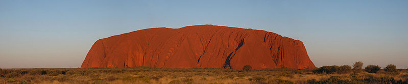
Figure: Uluru, the sacred rock in Australia. If we think of it as a probability density, viewing it from this side gives us one marginal from the density. Figuratively speaking, slicing through the rock would give a conditional density.

When viewing these contour plots, I sometimes find it helpful to think of Uluru, the prominent rock formation in Australia. The rock rises above the surface of the plane, just like a probability density rising above the zero line. The rock is three dimensional, but when we view Uluru from the classical position, we are looking at one side of it. This is equivalent to viewing the marginal density.

The joint density can be viewed from above, using contours. The conditional density is equivalent to slicing the rock. Uluru is a holy rock, so this has to be an imaginary slice. Imagine we cut down a vertical plane orthogonal to our view point (e.g. coming across our view point). This would give a profile of the rock, which when renormalized, would give us the conditional distribution, the value of conditioning would be the location of the slice in the direction we are facing.

Prediction of \(f_2\) from \(f_1\)

Of course in practice, rather than manipulating mountains physically, the advantage of the Gaussian density is that we can perform these manipulations mathematically.

Prediction of \(f_2\) given \(f_1\) requires the conditional density, \(p(f_2|f_1)\).Another remarkable property of the Gaussian density is that this conditional distribution is also guaranteed to be a Gaussian density. It has the form, \[ p(f_2|f_1) = \mathscr{N}\left(f_2|\frac{k_{1, 2}}{k_{1, 1}}f_1, k_{2, 2} - \frac{k_{1,2}^2}{k_{1,1}}\right) \]where we have assumed that the covariance of the original joint density was given by \[ \mathbf{K}= \begin{bmatrix} k_{1, 1} & k_{1, 2}\\ k_{2, 1} & k_{2, 2}.\end{bmatrix} \]

Using these formulae we can determine the conditional density for any of the elements of our vector \(\mathbf{ f}\). For example, the variable \(f_8\) is less correlated with \(f_1\) than \(f_2\). If we consider this variable we see the conditional density is more diffuse.

Joint Density of \(f_1\) and \(f_8\)

Figure: Sample from the joint Gaussian model, points indexed by 1 and 8 highlighted.

Prediction of \(f_{8}\) from \(f_{1}\)

Figure: The joint Gaussian over \(f_1\) and \(f_8\) along with the conditional distribution of \(f_8\) given \(f_1\)

• The single contour of the Gaussian density represents the joint distribution, \(p(f_1, f_8)\)

Where Did This Covariance Matrix Come From?

\[ k(\mathbf{ x}, \mathbf{ x}^\prime) = \alpha \exp\left(-\frac{\left\Vert \mathbf{ x}- \mathbf{ x}^\prime\right\Vert^2_2}{2\ell^2}\right)\]

import mlai

from mlai import Kernel

import mlai

from mlai import eq_cov

Figure: Entrywise fill in of the covariance matrix from the covariance function.

Figure: Entrywise fill in of the covariance matrix from the covariance function.

Figure: Entrywise fill in of the covariance matrix from the covariance function.

Thanks!

For more information on these subjects and more you might want to check the following resources.

• company: Trent AI
• book: The Atomic Human
• twitter: @lawrennd
• podcast: The Talking Machines
• newspaper: Guardian Profile Page
• blog: http://inverseprobability.com

References