Special Topics: Gaussian Processes

Review

• Last week: Logistic Regression and Generalised Linear Models
• Introduced link functions and different transformations.
• Showed examples in classification and mentioned possibilities for disease rate models.
• This week:
  • Gaussian Processes: non parametric Bayesian modelling

Generalized Linear Models

• Logistic regression is a generalized linear model
• Prediction function that is linear in parameters \[ \log \frac{p(\mathbf{ x})}{1-p(\mathbf{ x})} = f(\mathbf{ x}; \mathbf{ w}) \]
• Where \(f(\cdot)\) is linear in parameters.

Basis Functions

• Linear models have the form \[ f(\mathbf{ x}) = \mathbf{ w}^\top \boldsymbol{ \phi}(\mathbf{ x}). \]

• Gaussian processes are related to generalized linear models.

Gaussian Processes

• Basis function models give non-linear predictions.
• Need to choose number and location of basis functions.
• Gaussian processes is a general framework (basis functions special case)
• Within the framework you can consider models with infinite basis functions.

\[ p(\mathbf{ y}|\mathbf{X}, \mathbf{ w}) = \prod_{i=1}^{n} p(y_i | \mathbf{ x}_i, \mathbf{ w}) \]

\[ \mathbf{ y}|\mathbf{X}\sim \mathcal{N}\left(\mathbf{m}(\mathbf{X}),\mathbf{K}(\mathbf{X})\right), \]

Sampling a Function

Multi-variate Gaussians

• We will consider a Gaussian with a particular structure of covariance matrix.
• Generate a single sample from this 25 dimensional Gaussian density, \[ \mathbf{ f}=\left[f_{1},f_{2}\dots f_{25}\right]. \]
• We will plot these points against their index.

Gaussian Distribution Sample

❮ ❯

Sampling a Function from a Gaussian

❮ ❯

Joint Density of \(f_1\) and \(f_2\)

Prediction of \(f_{2}\) from \(f_{1}\)

❮ ❯

Uluru

Prediction with Correlated Gaussians

• Prediction of \(f_2\) from \(f_1\) requires conditional density.
• Conditional density is also Gaussian. \[ p(f_2|f_1) = \mathcal{N}\left(f_2|\frac{k_{1, 2}}{k_{1, 1}}f_1, k_{2, 2} - \frac{k_{1,2}^2}{k_{1,1}}\right) \] where covariance of joint density is given by \[ \mathbf{K}= \begin{bmatrix} k_{1, 1} & k_{1, 2}\\ k_{2, 1} & k_{2, 2}.\end{bmatrix} \]

Joint Density of \(f_1\) and \(f_8\)

Prediction of \(f_{8}\) from \(f_{1}\)

❮ ❯

Details

• The single contour of the Gaussian density represents the joint distribution, \(p(f_1, f_8)\)

Prediction with Correlated Gaussians

• Prediction of \(\mathbf{ f}_*\) from \(\mathbf{ f}\) requires multivariate conditional density.

• Multivariate conditional density is also Gaussian. \[ p(\mathbf{ f}_*|\mathbf{ f}) = {\mathcal{N}\left(\mathbf{ f}_*|\mathbf{K}_{*,\mathbf{ f}}\mathbf{K}_{\mathbf{ f},\mathbf{ f}}^{-1}\mathbf{ f},\mathbf{K}_{*,*}-\mathbf{K}_{*,\mathbf{ f}} \mathbf{K}_{\mathbf{ f},\mathbf{ f}}^{-1}\mathbf{K}_{\mathbf{ f},*}\right)} \]

• Here covariance of joint density is given by \[ \mathbf{K}= \begin{bmatrix} \mathbf{K}_{\mathbf{ f}, \mathbf{ f}} & \mathbf{K}_{*, \mathbf{ f}}\\ \mathbf{K}_{\mathbf{ f}, *} & \mathbf{K}_{*, *}\end{bmatrix} \]

Prediction with Correlated Gaussians

• Prediction of \(\mathbf{ f}_*\) from \(\mathbf{ f}\) requires multivariate conditional density.

• Multivariate conditional density is also Gaussian. \[ p(\mathbf{ f}_*|\mathbf{ f}) = {\mathcal{N}\left(\mathbf{ f}_*|\boldsymbol{ \mu},\boldsymbol{ \Sigma}\right)} \] \[ \boldsymbol{ \mu}= \mathbf{K}_{*,\mathbf{ f}}\mathbf{K}_{\mathbf{ f},\mathbf{ f}}^{-1}\mathbf{ f} \] \[ \boldsymbol{ \Sigma}= \mathbf{K}_{*,*}-\mathbf{K}_{*,\mathbf{ f}} \mathbf{K}_{\mathbf{ f},\mathbf{ f}}^{-1}\mathbf{K}_{\mathbf{ f},*} \]

• Here covariance of joint density is given by \[ \mathbf{K}= \begin{bmatrix} \mathbf{K}_{\mathbf{ f}, \mathbf{ f}} & \mathbf{K}_{*, \mathbf{ f}}\\ \mathbf{K}_{\mathbf{ f}, *} & \mathbf{K}_{*, *}\end{bmatrix} \]

Marginal Likelihood

Sampling from the Prior

Weight Space View

\[ \mathbf{ w}\sim \mathcal{N}\left(\mathbf{0},\alpha\mathbf{I}\right), \]

\[ f(\mathbf{ x}) = \mathbf{ w}^\top \boldsymbol{ \phi}(\mathbf{ x}). \]

Function Space View

\[ \mathbf{ w}\sim \mathcal{N}\left(\mathbf{0},\alpha \mathbf{I}\right) \]

\[ \boldsymbol{ \Phi}= \begin{bmatrix}\boldsymbol{ \phi}(\mathbf{ x}_1) \\ \vdots \\ \boldsymbol{ \phi}(\mathbf{ x}_n)\end{bmatrix} \]

\[ \mathbf{ f}= \begin{bmatrix} f_1 \\ \vdots f_n\end{bmatrix} \]

\[ \mathbf{ f}= \boldsymbol{ \Phi}\mathbf{ w}. \]

\[ \mathbf{ f}\sim \mathcal{N}\left(\mathbf{0},\alpha \boldsymbol{ \Phi}\boldsymbol{ \Phi}^\top\right). \]

\[ \mathbf{K}= \alpha \boldsymbol{ \Phi}\boldsymbol{ \Phi}^\top. \]

K = alpha*Phi_pred@Phi_pred.T

\[ \mathbf{ y}= \mathbf{ f}+ \boldsymbol{\epsilon} \]

\[ \epsilon \sim \mathcal{N}\left(\mathbf{0},\sigma^2\mathbf{I}\right). \]

\[ \mathbf{ y}\sim \mathcal{N}\left(\mathbf{0},\boldsymbol{ \Phi}\boldsymbol{ \Phi}^\top +\sigma^2\mathbf{I}\right). \]

Non-degenerate Gaussian Processes

• This process is degenerate.
• Covariance function is of rank at most \(h\).
• As \(n\rightarrow \infty\), covariance matrix is not full rank.
• Leading to \(\det{\mathbf{K}} = 0\)

Infinite Networks

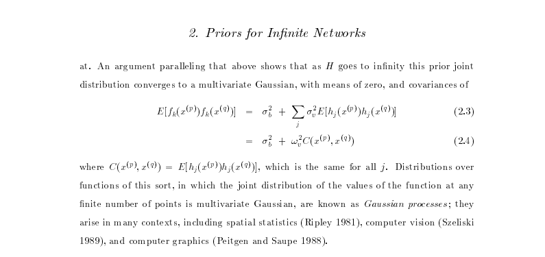
• In ML Radford Neal (Neal, 1994) asked “what would happen if you took \(h\rightarrow \infty\)?”

Roughly Speaking

• Instead of \[ \begin{align*} k_f\left(\mathbf{ x}_i, \mathbf{ x}_j\right) & = \alpha \boldsymbol{ \phi}\left(\mathbf{W}_1, \mathbf{ x}_i\right)^\top \boldsymbol{ \phi}\left(\mathbf{W}_1, \mathbf{ x}_j\right)\\ & = \alpha \sum_k \phi\left(\mathbf{ w}^{(1)}_k, \mathbf{ x}_i\right) \phi\left(\mathbf{ w}^{(1)}_k, \mathbf{ x}_j\right) \end{align*} \]
• Sample infinitely many from a prior density, \(p(\mathbf{ w}^{(1)})\), \[ k_f\left(\mathbf{ x}_i, \mathbf{ x}_j\right) = \alpha \int \phi\left(\mathbf{ w}^{(1)}, \mathbf{ x}_i\right) \phi\left(\mathbf{ w}^{(1)}, \mathbf{ x}_j\right) p(\mathbf{ w}^{(1)}) \text{d}\mathbf{ w}^{(1)} \]
• Also applies for non-Gaussian \(p(\mathbf{ w}^{(1)})\) because of the central limit theorem.

Simple Probabilistic Program

• If \[ \begin{align*} \mathbf{ w}^{(1)} & \sim p(\cdot)\\ \phi_i & = \phi\left(\mathbf{ w}^{(1)}, \mathbf{ x}_i\right), \end{align*} \] has finite variance.

• Then taking number of hidden units to infinity, is also a Gaussian process.

Further Reading

• Chapter 2 of Neal’s thesis (Neal, 1994)

• Rest of Neal’s thesis. (Neal, 1994)

• David MacKay’s PhD thesis (MacKay, 1992)

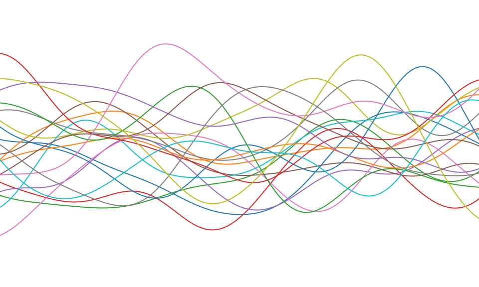
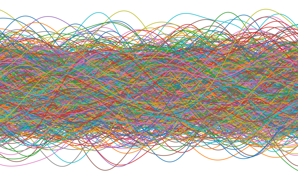
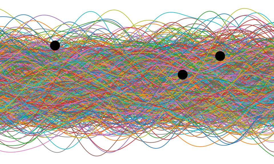
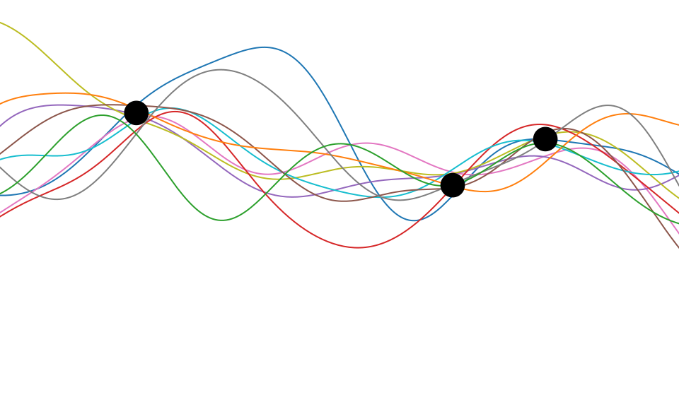
Gaussian Process

\[ k(\mathbf{ x}, \mathbf{ x}^\prime) = \alpha \exp\left( -\frac{\left\Vert \mathbf{ x}-\mathbf{ x}^\prime\right\Vert^2}{2\ell^2}\right), \]

\[ \left\Vert\mathbf{ x}- \mathbf{ x}^\prime\right\Vert^2 = (\mathbf{ x}- \mathbf{ x}^\prime)^\top (\mathbf{ x}- \mathbf{ x}^\prime) \]

Gaussian Process

\[ p(\mathbf{ y}|\mathbf{X}) = \frac{1}{(2\pi)^{\frac{n}{2}}|\mathbf{K}|^{\frac{1}{2}}} \exp\left(-\frac{1}{2}\mathbf{ y}^\top \left(\mathbf{K}+\sigma^2 \mathbf{I}\right)^{-1}\mathbf{ y}\right) \]

\[ E(\boldsymbol{\theta}) = \frac{1}{2} \log |\mathbf{K}| + \frac{1}{2} \mathbf{ y}^\top \left(\mathbf{K}+ \sigma^2\mathbf{I}\right)^{-1}\mathbf{ y} \]

Making Predictions

\[ \begin{bmatrix}\mathbf{ f}\\ \mathbf{ f}^*\end{bmatrix} \sim \mathcal{N}\left(\mathbf{0},\begin{bmatrix} \mathbf{K}& \mathbf{K}_\ast \\ \mathbf{K}_\ast^\top & \mathbf{K}_{\ast,\ast}\end{bmatrix}\right) \]

\[ \begin{bmatrix} \mathbf{K}& \mathbf{K}_\ast \\ \mathbf{K}_\ast^\top & \mathbf{K}_{\ast,\ast}\end{bmatrix} \]

The Importance of the Covariance Function

\[ \boldsymbol{ \mu}_f= \mathbf{A}^\top \mathbf{ y}, \]

Improving the Numerics

In practice we shouldn’t be using matrix inverse directly to solve the GP system. One more stable way is to compute the Cholesky decomposition of the kernel matrix. The log determinant of the covariance can also be derived from the Cholesky decomposition.

Capacity Control

Gradients of the Likelihood

Overall Process Scale

Capacity Control and Data Fit

Learning Covariance Parameters

Can we determine covariance parameters from the data?

\[ \mathcal{N}\left(\mathbf{ y}|\mathbf{0},\mathbf{K}\right)=\frac{1}{(2\pi)^\frac{n}{2}{\det{\mathbf{K}}^{\frac{1}{2}}}}{\exp\left(-\frac{\mathbf{ y}^{\top}\mathbf{K}^{-1}\mathbf{ y}}{2}\right)} \]

\[ \begin{aligned} \mathcal{N}\left(\mathbf{ y}|\mathbf{0},\mathbf{K}\right)=\frac{1}{(2\pi)^\frac{n}{2}\color{yellow}{\det{\mathbf{K}}^{\frac{1}{2}}}}\color{cyan}{\exp\left(-\frac{\mathbf{ y}^{\top}\mathbf{K}^{-1}\mathbf{ y}}{2}\right)} \end{aligned} \]

\[ \begin{aligned} \log \mathcal{N}\left(\mathbf{ y}|\mathbf{0},\mathbf{K}\right)=&\color{yellow}{-\frac{1}{2}\log\det{\mathbf{K}}}\color{cyan}{-\frac{\mathbf{ y}^{\top}\mathbf{K}^{-1}\mathbf{ y}}{2}} \\ &-\frac{n}{2}\log2\pi \end{aligned} \]

\[ E(\boldsymbol{ \theta}) = \color{yellow}{\frac{1}{2}\log\det{\mathbf{K}}} + \color{cyan}{\frac{\mathbf{ y}^{\top}\mathbf{K}^{-1}\mathbf{ y}}{2}} \]

Capacity Control through the Determinant

The parameters are inside the covariance function (matrix). \[k_{i, j} = k(\mathbf{ x}_i, \mathbf{ x}_j; \boldsymbol{ \theta})\]

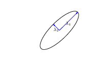
Eigendecomposition of Covariance

\[\mathbf{K}= \mathbf{R}\boldsymbol{ \Lambda}^2 \mathbf{R}^\top\]

\(\boldsymbol{ \Lambda}\) represents distance on axes. \(\mathbf{R}\) gives rotation.

Eigendecomposition of Covariance

• \(\boldsymbol{ \Lambda}\) is diagonal, \(\mathbf{R}^\top\mathbf{R}= \mathbf{I}\).
• Useful representation since \(\det{\mathbf{K}} = \det{\boldsymbol{ \Lambda}^2} = \det{\boldsymbol{ \Lambda}}^2\).

Capacity control: \(\color{yellow}{\log \det{\mathbf{K}}}\)

❮ ❯

Quadratic Data Fit

Data Fit: \(\color{cyan}{\frac{\mathbf{ y}^\top\mathbf{K}^{-1}\mathbf{ y}}{2}}\)

❮ ❯

\[E(\boldsymbol{ \theta}) = \color{yellow}{\frac{1}{2}\log\det{\mathbf{K}}}+\color{cyan}{\frac{\mathbf{ y}^{\top}\mathbf{K}^{-1}\mathbf{ y}}{2}}\]

Data Fit Term

❮ ❯

Exponentiated Quadratic Covariance

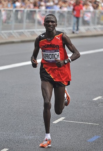
Olympic Marathon Data

Gold medal times for Olympic Marathon since 1896. Marathons before 1924 didn’t have a standardized distance. Present results using pace per km. In 1904 Marathon was badly organized leading to very slow times.

Image from Wikimedia Commons http://bit.ly/16kMKHQ

Olympic Marathon Data

Alan Turing

Probability Winning Olympics?

• He was a formidable Marathon runner.
• In 1946 he ran a time 2 hours 46 minutes.
  • That’s a pace of 3.95 min/km.
• What is the probability he would have won an Olympics if one had been held in 1946?

Gaussian Process Fit

Olympic Marathon Data GP

Della Gatta Gene Data

• Given given expression levels in the form of a time series from Della Gatta et al. (2008).

Della Gatta Gene Data

Gene Expression Example

• Want to detect if a gene is expressed or not, fit a GP to each gene Kalaitzis and Lawrence (2011).

TP53 Gene Data GP

TP53 Gene Data GP

TP53 Gene Data GP

Multiple Optima

Example: Prediction of Malaria Incidence in Uganda

• Work with Ricardo Andrade Pacheco, John Quinn and Martin Mubangizi (Makerere University, Uganda)
• See AI-DEV Group.
• See UN Global Pulse Disease Outbreaks Site

Malaria Prediction in Uganda

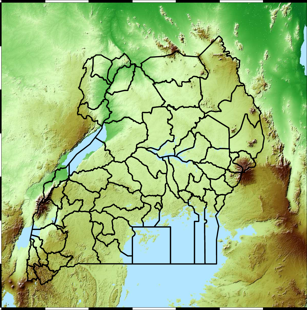
Kapchorwa District

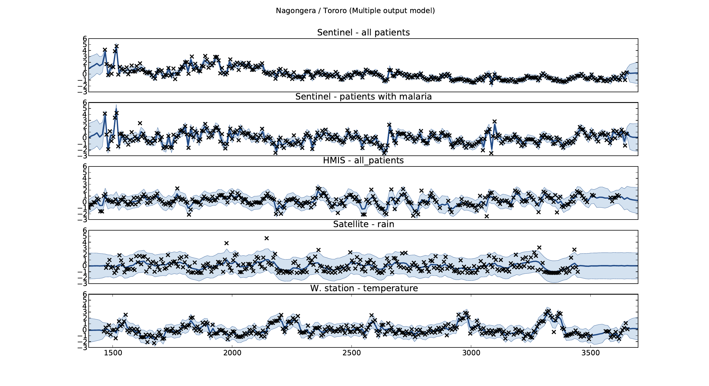
Tororo District

Malaria Prediction in Nagongera (Sentinel Site)

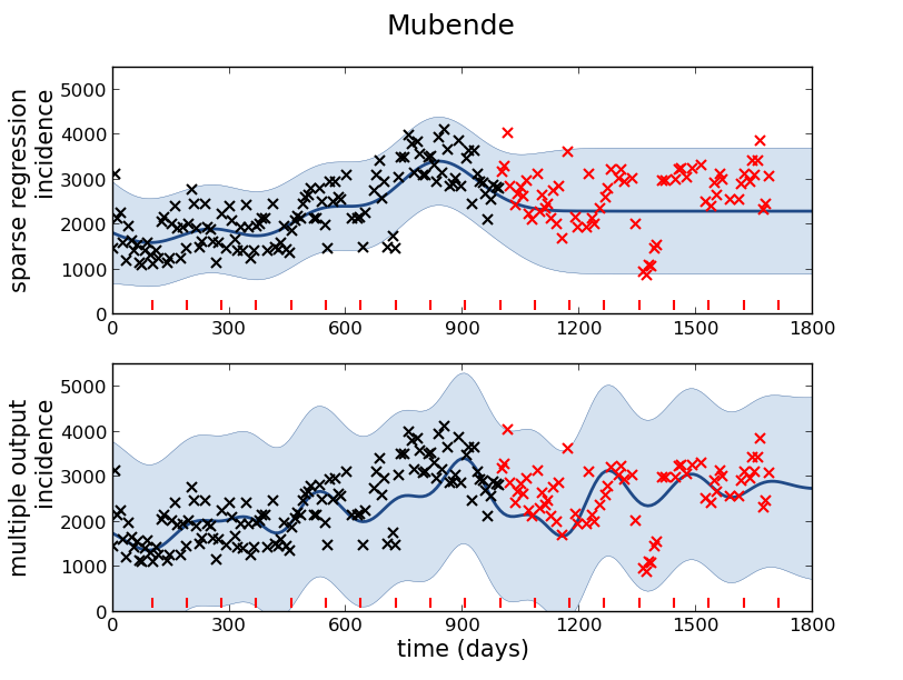
Mubende District

Malaria Prediction in Uganda

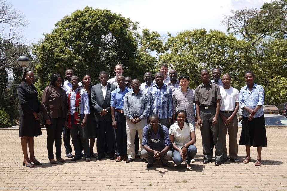
GP School at Makerere

Kabarole District

Early Warning System

Early Warning Systems

Additive Covariance

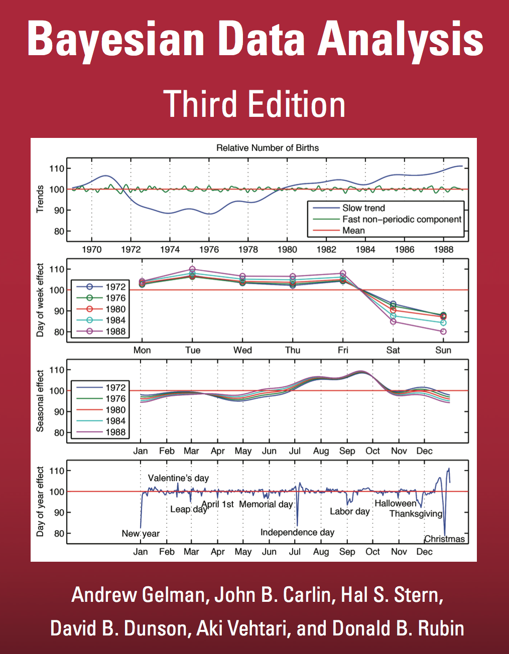
Gelman Book

Basis Function Covariance

Brownian Covariance

MLP Covariance

GPSS: Gaussian Process Summer School

GPy: A Gaussian Process Framework in Python

GPy: A Gaussian Process Framework in Python

• BSD Licensed software base.
• Wide availability of libraries, ‘modern’ scripting language.
• Allows us to set projects to undergraduates in Comp Sci that use GPs.
• Available through GitHub https://github.com/SheffieldML/GPy
• Reproducible Research with Jupyter Notebook.

Features

• Probabilistic-style programming (specify the model, not the algorithm).
• Non-Gaussian likelihoods.
• Multivariate outputs.
• Dimensionality reduction.
• Approximations for large data sets.