Probability and an Introduction to Jupyter, Python and Pandas
Course Texts
A First Course in Machine Learning
Additional Course Text
Pattern Recognition and Machine Learning
Assumed Knowledge
Choice of Language
Choice of Environment
What is Machine Learning?
What is Machine Learning?
\[ \text{data} + \text{model} \stackrel{\text{compute}}{\rightarrow} \text{prediction}\]
- data : observations, could be actively or passively acquired (meta-data).
- model : assumptions, based on previous experience (other data! transfer learning etc), or beliefs about the regularities of the universe. Inductive bias.
- prediction : an action to be taken or a categorization or a quality score.
- Royal Society Report: Machine Learning: Power and Promise of Computers that Learn by Example
What is Machine Learning?
\[\text{data} + \text{model} \stackrel{\text{compute}}{\rightarrow} \text{prediction}\]
- To combine data with a model need:
- a prediction function \(f(\cdot)\) includes our beliefs about the regularities of the universe
- an objective function \(E(\cdot)\) defines the cost of misprediction.
Overdetermined System
\(y= mx+ c\)
point 1: \(x= 1\), \(y=3\) \[ 3 = m + c \]
point 2: \(x= 3\), \(y=1\) \[ 1 = 3m + c \]
point 3: \(x= 2\), \(y=2.5\) \[ 2.5 = 2m + c \]
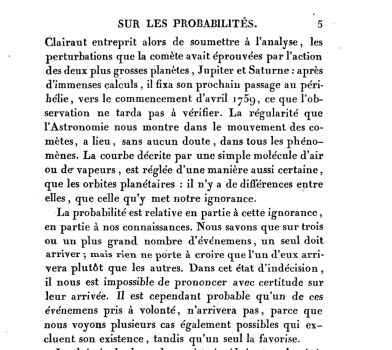
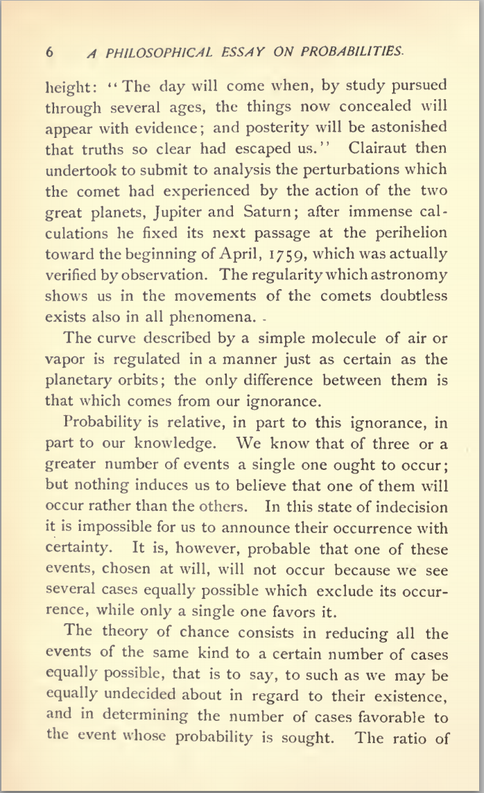
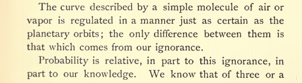
Pierre-Simon Laplace

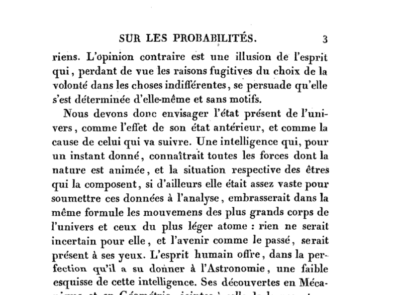
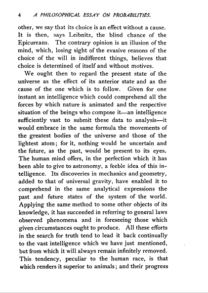
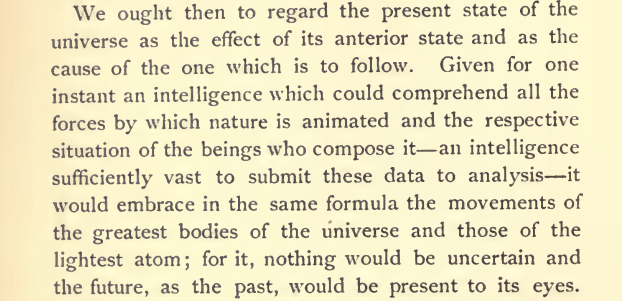
Laplace’s Gremlin
Latent Variables
\(y= mx+ c + \epsilon\)
point 1: \(x= 1\), \(y=3\) \[ 3 = m + c + \epsilon_1 \]
point 2: \(x= 3\), \(y=1\) \[ 1 = 3m + c + \epsilon_2 \]
point 3: \(x= 2\), \(y=2.5\) \[ 2.5 = 2m + c + \epsilon_3 \]
A Probabilistic Process
Set the mean of Gaussian to be a function. \[ p\left(y_i|x_i\right)=\frac{1}{\sqrt{2\pi\sigma^2}}\exp \left(-\frac{\left(y_i-f\left(x_i\right)\right)^{2}}{2\sigma^2}\right). \]
This gives us a ‘noisy function’.
This is known as a stochastic process.
Nigeria NMIS Data
Nigeria NMIS Data: Notebook

Probabilities
Exploring the NMIS Data
Probability and the NMIS Data
Conditioning
Probability Review
- We are interested in trials which result in two random variables, \(X\) and \(Y\), each of which has an ‘outcome’ denoted by \(x\) or \(y\).
- We summarise the notation and terminology for these distributions in the following table.
| Terminology | Mathematical notation | Description |
|---|---|---|
| joint | \(P(X=x, Y=y)\) | prob. that X=x and Y=y |
| marginal | \(P(X=x)\) | prob. that X=x regardless of Y |
| conditional | \(P(X=x\vert Y=y)\) | prob. that X=x given that Y=y |
A Pictorial Definition of Probability
Definition of probability distributions
| Terminology | Definition | Probability Notation |
|---|---|---|
| Joint Probability | \(\lim_{N\rightarrow\infty}\frac{n_{X=3,Y=4}}{N}\) | \(P\left(X=3,Y=4\right)\) |
| Marginal Probability | \(\lim_{N\rightarrow\infty}\frac{n_{X=5}}{N}\) | \(P\left(X=5\right)\) |
| Conditional Probability | \(\lim_{N\rightarrow\infty}\frac{n_{X=3,Y=4}}{n_{Y=4}}\) | \(P\left(X=3\vert Y=4\right)\) |
Notational Details
Typically we should write out \(P\left(X=x,Y=y\right)\).
In practice, we often use \(P\left(x,y\right)\).
This looks very much like we might write a multivariate function, e.g. \(f\left(x,y\right)=\frac{x}{y}\).
- For a multivariate function though, \(f\left(x,y\right)\neq f\left(y,x\right)\).
- However \(P\left(x,y\right)=P\left(y,x\right)\) because \(P\left(X=x,Y=y\right)=P\left(Y=y,X=x\right)\).
We now quickly review the ‘rules of probability’.
Normalization
All distributions are normalized. This is clear from the fact that \(\sum_{x}n_{x}=N\), which gives \[\sum_{x}P\left(x\right)={\lim_{N\rightarrow\infty}}\frac{\sum_{x}n_{x}}{N}={\lim_{N\rightarrow\infty}}\frac{N}{N}=1.\] A similar result can be derived for the marginal and conditional distributions.
The Product Rule
- \(P\left(x|y\right)\) is \[ {\lim_{N\rightarrow\infty}}\frac{n_{x,y}}{n_{y}}. \]
- \(P\left(x,y\right)\) is \[ {\lim_{N\rightarrow\infty}}\frac{n_{x,y}}{N}={\lim_{N\rightarrow\infty}}\frac{n_{x,y}}{n_{y}}\frac{n_{y}}{N} \] or in other words \[ P\left(x,y\right)=P\left(x|y\right)P\left(y\right). \] This is known as the product rule of probability.
The Sum Rule
Ignoring the limit in our definitions:
The marginal probability \(P\left(y\right)\) is \({\lim_{N\rightarrow\infty}}\frac{n_{y}}{N}\) .
The joint distribution \(P\left(x,y\right)\) is \({\lim_{N\rightarrow\infty}}\frac{n_{x,y}}{N}\).
\(n_{y}=\sum_{x}n_{x,y}\) so \[ {\lim_{N\rightarrow\infty}}\frac{n_{y}}{N}={\lim_{N\rightarrow\infty}}\sum_{x}\frac{n_{x,y}}{N}, \] in other words \[ P\left(y\right)=\sum_{x}P\left(x,y\right). \] This is known as the sum rule of probability.
Bayes’ Rule
- From the product rule, \[ P\left(y,x\right)=P\left(x,y\right)=P\left(x|y\right)P\left(y\right),\] so \[ P\left(y|x\right)P\left(x\right)=P\left(x|y\right)P\left(y\right) \] which leads to Bayes’ rule, \[ P\left(y|x\right)=\frac{P\left(x|y\right)P\left(y\right)}{P\left(x\right)}. \]
Bayes’ Theorem Example
- There are two barrels in front of you. Barrel One contains 20 apples and 4 oranges. Barrel Two other contains 4 apples and 8 oranges. You choose a barrel randomly and select a fruit. It is an apple. What is the probability that the barrel was Barrel One?
Bayes’ Rule Example: Answer I
- We are given that: \[\begin{aligned} P(\text{F}=\text{A}|\text{B}=1) = & 20/24 \\ P(\text{F}=\text{A}|\text{B}=2) = & 4/12 \\ P(\text{B}=1) = & 0.5 \\ P(\text{B}=2) = & 0.5 \end{aligned}\]
Bayes’ Rule Example: Answer II
- We use the sum rule to compute: \[\begin{aligned} P(\text{F}=\text{A}) = & P(\text{F}=\text{A}|\text{B}=1)P(\text{B}=1) \\& + P(\text{F}=\text{A}|\text{B}=2)P(\text{B}=2) \\ = & 20/24\times 0.5 + 4/12 \times 0.5 = 7/12 \end{aligned}\]
- And Bayes’ rule tells us that: \[\begin{aligned} P(\text{B}=1|\text{F}=\text{A}) = & \frac{P(\text{F} = \text{A}|\text{B}=1)P(\text{B}=1)}{P(\text{F}=\text{A})}\\ = & \frac{20/24 \times 0.5}{7/12} = 5/7 \end{aligned}\]
Further Reading
- Probability distributions: page 12–17 (Section 1.2) of Bishop (2006)
Exercises
- Exercise 1.3 of Bishop (2006)
Computing Expectations Example
- Consider the following distribution.
| \(y\) | 1 | 2 | 3 | 4 |
|---|---|---|---|---|
| \(P\left(y\right)\) | 0.3 | 0.2 | 0.1 | 0.4 |
- What is the mean of the distribution?
- What is the standard deviation of the distribution?
- Are the mean and standard deviation representative of the distribution form?
- What is the expected value of \(-\log P(y)\)?
Expectations Example: Answer
- We are given that:
| \(y\) | 1 | 2 | 3 | 4 |
|---|---|---|---|---|
| \(P\left(y\right)\) | 0.3 | 0.2 | 0.1 | 0.4 |
| \(y^2\) | 1 | 4 | 9 | 16 |
| \(-\log(P(y))\) | 1.204 | 1.609 | 2.302 | 0.916 |
- Mean: \(1\times 0.3 + 2\times 0.2 + 3 \times 0.1 + 4 \times 0.4 = 2.6\)
- Second moment: \(1 \times 0.3 + 4 \times 0.2 + 9 \times 0.1 + 16 \times 0.4 = 8.4\)
- Variance: \(8.4 - 2.6\times 2.6 = 1.64\)
- Standard deviation: \(\sqrt{1.64} = 1.2806\)
Expectations Example: Answer II
- We are given that:
| \(y\) | 1 | 2 | 3 | 4 |
|---|---|---|---|---|
| \(P\left(y\right)\) | 0.3 | 0.2 | 0.1 | 0.4 |
| \(y^2\) | 1 | 4 | 9 | 16 |
| \(-\log(P(y))\) | 1.204 | 1.609 | 2.302 | 0.916 |
- Expectation \(-\log(P(y))\): \(0.3\times 1.204 + 0.2\times 1.609 + 0.1\times 2.302 +0.4\times 0.916 = 1.280\)
Sample Based Approximation Example
You are given the following values samples of heights of students,
\(i\) 1 2 3 4 5 6 \(y_i\) 1.76 1.73 1.79 1.81 1.85 1.80 What is the sample mean?
What is the sample variance?
Can you compute sample approximation expected value of \(-\log P(y)\)?
Sample Based Approximation Example: Answer
- We can compute:
| \(i\) | 1 | 2 | 3 | 4 | 5 | 6 |
|---|---|---|---|---|---|---|
| \(y_i\) | 1.76 | 1.73 | 1.79 | 1.81 | 1.85 | 1.80 |
| \(y^2_i\) | 3.0976 | 2.9929 | 3.2041 | 3.2761 | 3.4225 | 3.2400 |
- Mean: \(\frac{1.76 + 1.73 + 1.79 + 1.81 + 1.85 + 1.80}{6} = 1.79\)
- Second moment: $ = 3.2055$
- Variance: \(3.2055 - 1.79\times1.79 = 1.43\times 10^{-3}\)
- Standard deviation: \(0.0379\)
- No, you can’t compute it. You don’t have access to \(P(y)\) directly.
Sample Based Approximation Example
You are given the following values samples of heights of students,
\(i\) 1 2 3 4 5 6 \(y_i\) 1.76 1.73 1.79 1.81 1.85 1.80 Actually these “data” were sampled from a Gaussian with mean 1.7 and standard deviation 0.15. Are your estimates close to the real values? If not why not?
Reading
See probability review at end of slides for reminders.
For other material in Bishop read:
If you are unfamiliar with probabilities you should complete the following exercises:
Thanks!
book: The Atomic Human
twitter: @lawrennd
podcast: The Talking Machines
newspaper: Guardian Profile Page
blog posts:
Further Reading
Section 2.2 (pg 41–53) of Rogers and Girolami (2011)
Section 2.4 (pg 55–58) of Rogers and Girolami (2011)
Section 2.5.1 (pg 58–60) of Rogers and Girolami (2011)
Section 2.5.3 (pg 61–62) of Rogers and Girolami (2011)
Probability densities: Section 1.2.1 (Pages 17–19) of Bishop (2006)
Expectations and Covariances: Section 1.2.2 (Pages 19–20) of Bishop (2006)
The Gaussian density: Section 1.2.4 (Pages 24–28) (don’t worry about material on bias) of Bishop (2006)
For material on information theory and KL divergence try Section 1.6 & 1.6.1 (pg 48 onwards) of Bishop (2006)
Exercises
Exercise 1.7 of Bishop (2006)
Exercise 1.8 of Bishop (2006)
Exercise 1.9 of Bishop (2006)