Deep Gaussian Processes I
Structure of Priors
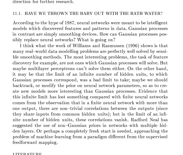
MacKay: NeurIPS Tutorial 1997 “Have we thrown out the baby with the bathwater?” (Published as MacKay, n.d.)
Deep Neural Network
Deep Neural Network
Mathematically
\[ \begin{align*} \mathbf{ h}_{1} &= \phi\left(\mathbf{W}_1 \mathbf{ x}\right)\\ \mathbf{ h}_{2} &= \phi\left(\mathbf{W}_2\mathbf{ h}_{1}\right)\\ \mathbf{ h}_{3} &= \phi\left(\mathbf{W}_3 \mathbf{ h}_{2}\right)\\ f&= \mathbf{ w}_4 ^\top\mathbf{ h}_{3} \end{align*} \]
Overfitting
Potential problem: if number of nodes in two adjacent layers is big, corresponding \(\mathbf{W}\) is also very big and there is the potential to overfit.
Proposed solution: “dropout”.
Alternative solution: parameterize \(\mathbf{W}\) with its SVD. \[ \mathbf{W}= \mathbf{U}\boldsymbol{ \Lambda}\mathbf{V}^\top \] or \[ \mathbf{W}= \mathbf{U}\mathbf{V}^\top \] where if \(\mathbf{W}\in \Re^{k_1\times k_2}\) then \(\mathbf{U}\in \Re^{k_1\times q}\) and \(\mathbf{V}\in \Re^{k_2\times q}\), i.e. we have a low rank matrix factorization for the weights.
Low Rank Approximation
Bottleneck Layers in Deep Neural Networks
Deep Neural Network
Mathematically
The network can now be written mathematically as \[ \begin{align} \mathbf{ z}_{1} &= \mathbf{V}^\top_1 \mathbf{ x}\\ \mathbf{ h}_{1} &= \phi\left(\mathbf{U}_1 \mathbf{ z}_{1}\right)\\ \mathbf{ z}_{2} &= \mathbf{V}^\top_2 \mathbf{ h}_{1}\\ \mathbf{ h}_{2} &= \phi\left(\mathbf{U}_2 \mathbf{ z}_{2}\right)\\ \mathbf{ z}_{3} &= \mathbf{V}^\top_3 \mathbf{ h}_{2}\\ \mathbf{ h}_{3} &= \phi\left(\mathbf{U}_3 \mathbf{ z}_{3}\right)\\ \mathbf{ y}&= \mathbf{ w}_4^\top\mathbf{ h}_{3}. \end{align} \]
A Cascade of Neural Networks
\[ \begin{align} \mathbf{ z}_{1} &= \mathbf{V}^\top_1 \mathbf{ x}\\ \mathbf{ z}_{2} &= \mathbf{V}^\top_2 \phi\left(\mathbf{U}_1 \mathbf{ z}_{1}\right)\\ \mathbf{ z}_{3} &= \mathbf{V}^\top_3 \phi\left(\mathbf{U}_2 \mathbf{ z}_{2}\right)\\ \mathbf{ y}&= \mathbf{ w}_4 ^\top \mathbf{ z}_{3} \end{align} \]
Cascade of Gaussian Processes
Replace each neural network with a Gaussian process \[ \begin{align} \mathbf{ z}_{1} &= \mathbf{ f}_1\left(\mathbf{ x}\right)\\ \mathbf{ z}_{2} &= \mathbf{ f}_2\left(\mathbf{ z}_{1}\right)\\ \mathbf{ z}_{3} &= \mathbf{ f}_3\left(\mathbf{ z}_{2}\right)\\ \mathbf{ y}&= \mathbf{ f}_4\left(\mathbf{ z}_{3}\right) \end{align} \]
Equivalent to prior over parameters, take width of each layer to infinity.
Deep Learning
Outline of the DeepFace architecture. A front-end of a single convolution-pooling-convolution filtering on the rectified input, followed by three locally-connected layers and two fully-connected layers. Color illustrates feature maps produced at each layer. The net includes more than 120 million parameters, where more than 95% come from the local and fully connected.


Mathematically
Composite multivariate function
\[ \mathbf{g}(\mathbf{ x})=\mathbf{ f}_5(\mathbf{ f}_4(\mathbf{ f}_3(\mathbf{ f}_2(\mathbf{ f}_1(\mathbf{ x}))))). \]
Equivalent to Markov Chain
- Composite multivariate function \[ p(\mathbf{ y}|\mathbf{ x})= p(\mathbf{ y}|\mathbf{ f}_5)p(\mathbf{ f}_5|\mathbf{ f}_4)p(\mathbf{ f}_4|\mathbf{ f}_3)p(\mathbf{ f}_3|\mathbf{ f}_2)p(\mathbf{ f}_2|\mathbf{ f}_1)p(\mathbf{ f}_1|\mathbf{ x}) \]
Why Composition?
Gaussian processes give priors over functions.
Elegant properties:
- e.g. Derivatives of process are also Gaussian distributed (if they exist).
For particular covariance functions they are ‘universal approximators’, i.e. all functions can have support under the prior.
Gaussian derivatives might ring alarm bells.
E.g. a priori they don’t believe in function ‘jumps’.
Stochastic Process Composition
From a process perspective: process composition.
A (new?) way of constructing more complex processes based on simpler components.
Difficulty for Probabilistic Approaches
Propagate a probability distribution through a non-linear mapping.
Normalisation of distribution becomes intractable.
Difficulty for Probabilistic Approaches
Propagate a probability distribution through a non-linear mapping.
Normalisation of distribution becomes intractable.
Difficulty for Probabilistic Approaches
Propagate a probability distribution through a non-linear mapping.
Normalisation of distribution becomes intractable.
Standard Variational Approach Fails
- Standard variational bound has the form: \[ \mathcal{L}= \left\langle\log p(\mathbf{ y}|\mathbf{Z})\right\rangle_{q(\mathbf{Z})} + \text{KL}\left( q(\mathbf{Z})\,\|\,p(\mathbf{Z}) \right) \]
Standard Variational Approach Fails
- Requires expectation of \(\log p(\mathbf{ y}|\mathbf{Z})\) under \(q(\mathbf{Z})\). \[ \begin{align} \log p(\mathbf{ y}|\mathbf{Z}) = & -\frac{1}{2}\mathbf{ y}^\top\left(\mathbf{K}_{\mathbf{ f}, \mathbf{ f}}+\sigma^2\mathbf{I}\right)^{-1}\mathbf{ y}\\ & -\frac{1}{2}\log \det{\mathbf{K}_{\mathbf{ f}, \mathbf{ f}}+\sigma^2 \mathbf{I}} -\frac{n}{2}\log 2\pi \end{align} \] \(\mathbf{K}_{\mathbf{ f}, \mathbf{ f}}\) is dependent on \(\mathbf{Z}\) and it appears in the inverse.
Variational Bayesian GP-LVM
- Consider collapsed variational bound, \[ p(\mathbf{ y})\geq \prod_{i=1}^nc_i \int \mathcal{N}\left(\mathbf{ y}|\left\langle\mathbf{ f}\right\rangle,\sigma^2\mathbf{I}\right)p(\mathbf{ u}) \text{d}\mathbf{ u} \] \[ p(\mathbf{ y}|\mathbf{Z})\geq \prod_{i=1}^nc_i \int \mathcal{N}\left(\mathbf{ y}|\left\langle\mathbf{ f}\right\rangle_{p(\mathbf{ f}|\mathbf{ u}, \mathbf{Z})},\sigma^2\mathbf{I}\right)p(\mathbf{ u}) \text{d}\mathbf{ u} \] \[ \int p(\mathbf{ y}|\mathbf{Z})p(\mathbf{Z}) \text{d}\mathbf{Z}\geq \int \prod_{i=1}^nc_i \mathcal{N}\left(\mathbf{ y}|\left\langle\mathbf{ f}\right\rangle_{p(\mathbf{ f}|\mathbf{ u}, \mathbf{Z})},\sigma^2\mathbf{I}\right) p(\mathbf{Z})\text{d}\mathbf{Z}p(\mathbf{ u}) \text{d}\mathbf{ u} \]
Variational Bayesian GP-LVM
- Apply variational lower bound to the inner integral. \[ \begin{align} \int \prod_{i=1}^nc_i \mathcal{N}\left(\mathbf{ y}|\left\langle\mathbf{ f}\right\rangle_{p(\mathbf{ f}|\mathbf{ u}, \mathbf{Z})},\sigma^2\mathbf{I}\right) p(\mathbf{Z})\text{d}\mathbf{Z}\geq & \left\langle\sum_{i=1}^n\log c_i\right\rangle_{q(\mathbf{Z})}\\ & +\left\langle\log\mathcal{N}\left(\mathbf{ y}|\left\langle\mathbf{ f}\right\rangle_{p(\mathbf{ f}|\mathbf{ u}, \mathbf{Z})},\sigma^2\mathbf{I}\right)\right\rangle_{q(\mathbf{Z})}\\& + \text{KL}\left( q(\mathbf{Z})\,\|\,p(\mathbf{Z}) \right) \end{align} \]
- Which is analytically tractable for Gaussian \(q(\mathbf{Z})\) and some covariance functions.
Required Expectations
- Need expectations under \(q(\mathbf{Z})\) of: \[ \log c_i = \frac{1}{2\sigma^2} \left[k_{i, i} - \mathbf{ k}_{i, \mathbf{ u}}^\top \mathbf{K}_{\mathbf{ u}, \mathbf{ u}}^{-1} \mathbf{ k}_{i, \mathbf{ u}}\right] \] and \[ \log \mathcal{N}\left(\mathbf{ y}|\left\langle\mathbf{ f}\right\rangle_{p(\mathbf{ f}|\mathbf{ u},\mathbf{Y})},\sigma^2\mathbf{I}\right) = -\frac{1}{2}\log 2\pi\sigma^2 - \frac{1}{2\sigma^2}\left(y_i - \mathbf{K}_{\mathbf{ f}, \mathbf{ u}}\mathbf{K}_{\mathbf{ u},\mathbf{ u}}^{-1}\mathbf{ u}\right)^2 \]
Required Expectations
- This requires the expectations \[ \left\langle\mathbf{K}_{\mathbf{ f},\mathbf{ u}}\right\rangle_{q(\mathbf{Z})} \] and \[ \left\langle\mathbf{K}_{\mathbf{ f},\mathbf{ u}}\mathbf{K}_{\mathbf{ u},\mathbf{ u}}^{-1}\mathbf{K}_{\mathbf{ u},\mathbf{ f}}\right\rangle_{q(\mathbf{Z})} \] which can be computed analytically for some covariance functions (Damianou et al., 2016) or through sampling (Damianou, 2015; Salimbeni and Deisenroth, 2017).
See also …
- MAP approach (Lawrence and Moore, 2007).
- Hamiltonian Monte Carlo approach (Havasi et al., 2018).
- Expectation Propagation approach (Bui et al., 2016).
Neural Networks
Deep Gaussian Processes
- Deep architectures allow abstraction of features (Bengio, 2009; Hinton and Osindero, 2006; Salakhutdinov and Murray, n.d.)
- We use variational approach to stack GP models.
Stacked PCA
Stacked GP
Analysis of Deep GPs
Avoiding pathologies in very deep networks Duvenaud et al. (2014) show that the derivative distribution of the process becomes more heavy tailed as number of layers increase.
How Deep Are Deep Gaussian Processes? Dunlop et al. (n.d.) perform a theoretical analysis possible through conditional Gaussian Markov property.
Stacked GPs (video by David Duvenaud)
GPy: A Gaussian Process Framework in Python
GPy: A Gaussian Process Framework in Python
- BSD Licensed software base.
- Wide availability of libraries, ‘modern’ scripting language.
- Allows us to set projects to undergraduates in Comp Sci that use GPs.
- Available through GitHub https://github.com/SheffieldML/GPy
- Reproducible Research with Jupyter Notebook.
Features
- Probabilistic-style programming (specify the model, not the algorithm).
- Non-Gaussian likelihoods.
- Multivariate outputs.
- Dimensionality reduction.
- Approximations for large data sets.
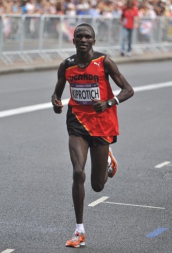
Olympic Marathon Data
|
|
Olympic Marathon Data
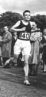
Alan Turing

|
|
Probability Winning Olympics?
- He was a formidable Marathon runner.
- In 1946 he ran a time 2 hours 46 minutes.
- That’s a pace of 3.95 min/km.
- What is the probability he would have won an Olympics if one had been held in 1946?
Gaussian Process Fit
Olympic Marathon Data GP
Deep GP Fit
Can a Deep Gaussian process help?
Deep GP is one GP feeding into another.
Olympic Marathon Data Deep GP
Olympic Marathon Data Deep GP
Olympic Marathon Data Latent 1
Olympic Marathon Data Latent 2
Olympic Marathon Pinball Plot
Della Gatta Gene Data
- Given given expression levels in the form of a time series from Della Gatta et al. (2008).
Della Gatta Gene Data
Gene Expression Example
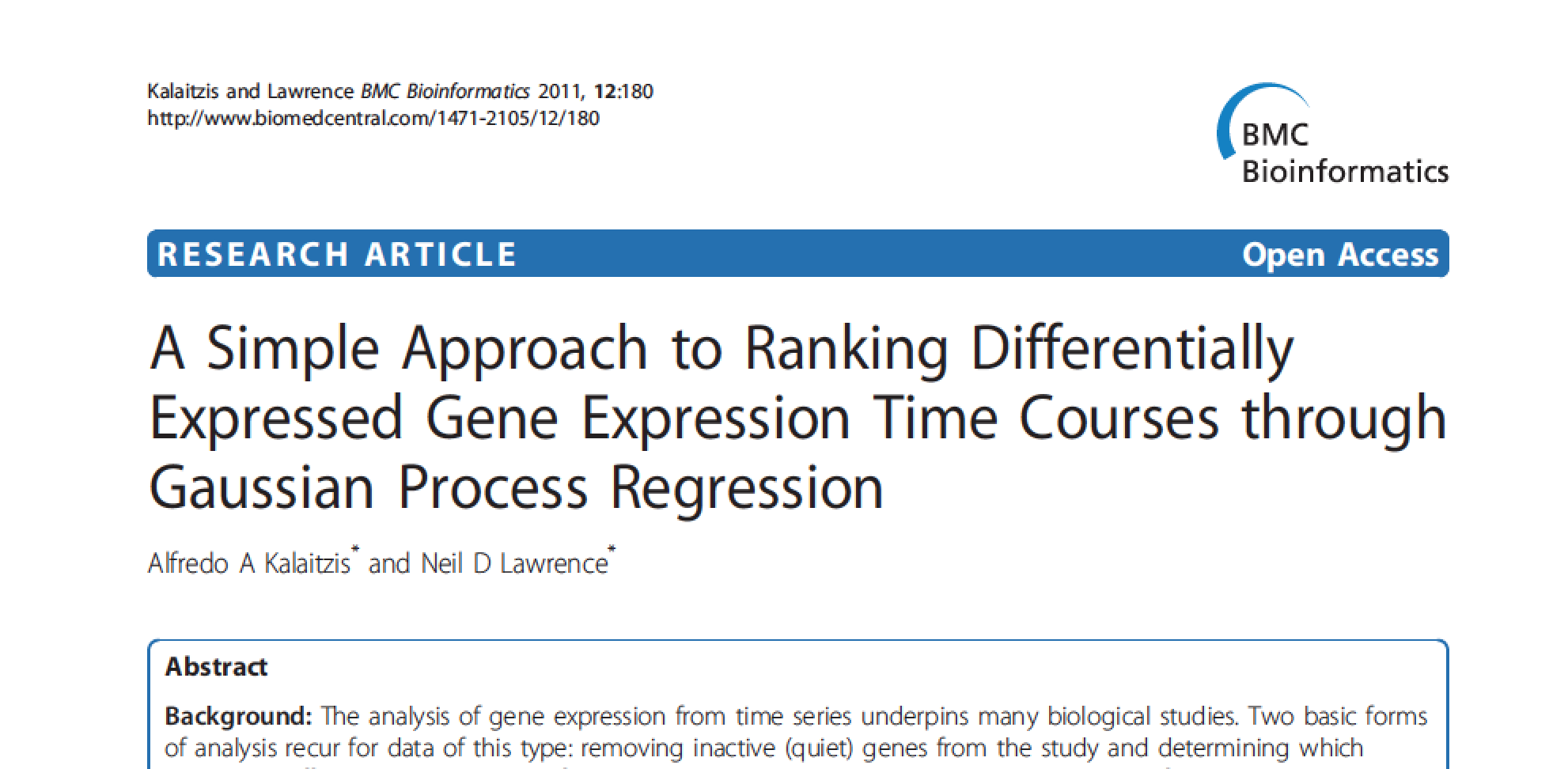
- Want to detect if a gene is expressed or not, fit a GP to each gene Kalaitzis and Lawrence (2011).
TP53 Gene Data GP
TP53 Gene Data GP
TP53 Gene Data GP
Multiple Optima
Della Gatta Gene Data Deep GP
Della Gatta Gene Data Deep GP
Della Gatta Gene Data Latent 1
Della Gatta Gene Data Latent 2
TP53 Gene Pinball Plot
Step Function Data
Step Function Data GP
Step Function Data Deep GP
Step Function Data Deep GP
Step Function Data Latent 1
Step Function Data Latent 2
Step Function Data Latent 3
Step Function Data Latent 4
Step Function Pinball Plot
Motorcycle Helmet Data
Motorcycle Helmet Data GP
Motorcycle Helmet Data Deep GP
Motorcycle Helmet Data Deep GP
Motorcycle Helmet Data Latent 1
Motorcycle Helmet Data Latent 2
Motorcycle Helmet Pinball Plot
Thanks!
- twitter: @lawrennd
- podcast: The Talking Machines
- newspaper: Guardian Profile Page
- blog: http://inverseprobability.com