Approximate Gaussian Processes

GPy: A Gaussian Process Framework in Python

https://github.com/SheffieldML/GPy

GPy: A Gaussian Process Framework in Python

BSD Licensed software base.
Wide availability of libraries, ‘modern’ scripting language.
Allows us to set projects to undergraduates in Comp Sci that use GPs.
Available through GitHub https://github.com/SheffieldML/GPy
Reproducible Research with Jupyter Notebook.

Features

Probabilistic-style programming (specify the model, not the algorithm).
Non-Gaussian likelihoods.
Multivariate outputs.
Dimensionality reduction.
Approximations for large data sets.

Approximations

Figure: Image credit: Kai Arulkumaran

Approximations

Figure: Image credit: Kai Arulkumaran

Approximations

Figure: Image credit: Kai Arulkumaran

Approximations

Figure: Image credit: Kai Arulkumaran

Approximate Gaussian Processes

Low Rank Motivation

Inference in a GP has the following demands:

Complexity: $\mathcal{O}(n^3)$

Storage: $\mathcal{O}(n^2)$
Inference in a low rank GP has the following demands:

Complexity: $\mathcal{O}(nm^2)$

Storage: $\mathcal{O}(nm)$

where $m$ is a user chosen parameter.

Snelson and Ghahramani (n.d.),Quiñonero Candela and Rasmussen (2005),Lawrence (n.d.),Titsias (n.d.),Bui et al. (2017)

Variational Compression

Inducing variables are a compression of the real observations.
They are like pseudo-data. They can be in space of $\mathbf{ f}$ or a space that is related through a linear operator (Álvarez et al., 2010) — e.g. a gradient or convolution.

Variational Compression II

Introduce inducing variables.
Compress information into the inducing variables and avoid the need to store all the data.
Allow for scaling e.g. stochastic variational Hensman et al. (n.d.) or parallelization Gal et al. (n.d.),Dai et al. (2014), Seeger et al. (2017)

Nonparametric Gaussian Processes

We’ve seen how we go from parametric to non-parametric.
The limit implies infinite dimensional $\mathbf{ w}$ .
Gaussian processes are generally non-parametric: combine data with covariance function to get model.
This representation cannot be summarized by a parameter vector of a fixed size.

The Parametric Bottleneck

Parametric models have a representation that does not respond to increasing training set size.
Bayesian posterior distributions over parameters contain the information about the training data.
- Use Bayes’ rule from training data, $p\left(\mathbf{ w}|\mathbf{ y}, \mathbf{X}\right)$ ,
- Make predictions on test data $p\left(y_*|\mathbf{X}_*, \mathbf{ y}, \mathbf{X}\right) = \int p\left(y_*|\mathbf{ w},\mathbf{X}_*\right)p\left(\mathbf{ w}|\mathbf{ y}, \mathbf{X})\text{d}\mathbf{ w}\right).$
$\mathbf{ w}$ becomes a bottleneck for information about the training set to pass to the test set.
Solution: increase $m$ so that the bottleneck is so large that it no longer presents a problem.
How big is big enough for $m$ ? Non-parametrics says $m\rightarrow \infty$ .

The Parametric Bottleneck

Now no longer possible to manipulate the model through the standard parametric form.

However, it is possible to express parametric as GPs: $k\left(\mathbf{ x}_i,\mathbf{ x}_j\right)=\phi_:\left(\mathbf{ x}_i\right)^\top\phi_:\left(\mathbf{ x}_j\right).$

These are known as degenerate covariance matrices.

Their rank is at most $m$ , non-parametric models have full rank covariance matrices.

Most well known is the “linear kernel”, $k(\mathbf{ x}_i, \mathbf{ x}_j) = \mathbf{ x}_i^\top\mathbf{ x}_j$ .

Making Predictions

For non-parametrics prediction at new points $\mathbf{ f}_*$ is made by conditioning on $\mathbf{ f}$ in the joint distribution.

In GPs this involves combining the training data with the covariance function and the mean function.

Parametric is a special case when conditional prediction can be summarized in a fixed number of parameters.

Complexity of parametric model remains fixed regardless of the size of our training data set.

For a non-parametric model the required number of parameters grows with the size of the training data.

Information capture

Everything we want to do with a GP involves marginalising $\mathbf{ f}$
- Predictions
- Marginal likelihood
- Estimating covariance parameters
The posterior of $\mathbf{ f}$ is the central object. This means inverting $\mathbf{K}_{\mathbf{ f}\mathbf{ f}}$ .

Nystr"om Method

Figure: Figure originally from presentation by Ed Snelson at NIPS

$\mathbf{K}_{\mathbf{ f}\mathbf{ f}}\approx \mathbf{Q}_{\mathbf{ f}\mathbf{ f}}= \mathbf{K}_{\mathbf{ f}\mathbf{ u}}\mathbf{K}_{\mathbf{ u}\mathbf{ u}}^{-1}\mathbf{K}_{\mathbf{ u}\mathbf{ f}}$

$\mathbf{X},\,\mathbf{ y}$

${\color{yellow} f(\mathbf{ x})} \sim {\mathcal GP}$

$\mathbf{X},\,\mathbf{ y}$

$f(\mathbf{ x}) \sim {\mathcal GP}$

$p({\color{yellow} \mathbf{ f}}) = \mathcal{N}\left(\mathbf{0},\mathbf{K}_{\mathbf{ f}\mathbf{ f}}\right)$

$\mathbf{X},\,\mathbf{ y}$

$f(\mathbf{ x}) \sim {\mathcal GP}$

$p(\mathbf{ f}) = \mathcal{N}\left(\mathbf{0},\mathbf{K}_{\mathbf{ f}\mathbf{ f}}\right)$

$p( \mathbf{ f}|\mathbf{ y},\mathbf{X})$

Introducing $\mathbf{ u}$

Take an extra $m$ points on the function, $\mathbf{ u}= f(\mathbf{Z})$ . $p(\mathbf{ y},\mathbf{ f},\mathbf{ u}) = p(\mathbf{ y}|\mathbf{ f}) p(\mathbf{ f}|\mathbf{ u}) p(\mathbf{ u})$

Introducing $\mathbf{ u}$

Take and extra $M$ points on the function, $\mathbf{ u}= f(\mathbf{Z})$ . $p(\mathbf{ y},\mathbf{ f},\mathbf{ u}) = p(\mathbf{ y}|\mathbf{ f}) p(\mathbf{ f}|\mathbf{ u}) p(\mathbf{ u})$ $\begin{aligned} p(\mathbf{ y}|\mathbf{ f}) &= \mathcal{N}\left(\mathbf{ y}|\mathbf{ f},\sigma^2 \mathbf{I}\right)\\ p(\mathbf{ f}|\mathbf{ u}) &= \mathcal{N}\left(\mathbf{ f}| \mathbf{K}_{\mathbf{ f}\mathbf{ u}}\mathbf{K}_{\mathbf{ u}\mathbf{ u}}^{-1}\mathbf{ u}, \tilde{\mathbf{K}}\right)\\ p(\mathbf{ u}) &= \mathcal{N}\left(\mathbf{ u}| \mathbf{0},\mathbf{K}_{\mathbf{ u}\mathbf{ u}}\right) \end{aligned}$

$\mathbf{X},\,\mathbf{ y}$

$f(\mathbf{ x}) \sim {\mathcal GP}$

$p(\mathbf{ f}) = \mathcal{N}\left(\mathbf{0},\mathbf{K}_{\mathbf{ f}\mathbf{ f}}\right)$

$p(\mathbf{ f}|\mathbf{ y},\mathbf{X})$

$\begin{align} &\qquad\mathbf{Z}, \mathbf{ u}\\ &p({\color{red} \mathbf{ u}}) = \mathcal{N}\left(\mathbf{0},\mathbf{K}_{\mathbf{ u}\mathbf{ u}}\right)\end{align}$

$\mathbf{X},\,\mathbf{ y}$

$f(\mathbf{ x}) \sim {\mathcal GP}$

$p(\mathbf{ f}) = \mathcal{N}\left(\mathbf{0},\mathbf{K}_{\mathbf{ f}\mathbf{ f}}\right)$

$p(\mathbf{ f}|\mathbf{ y},\mathbf{X})$

$p(\mathbf{ u}) = \mathcal{N}\left(\mathbf{0},\mathbf{K}_{\mathbf{ u}\mathbf{ u}}\right)$

$\widetilde p({\color{red}\mathbf{ u}}|\mathbf{ y},\mathbf{X})$

The alternative posterior

Instead of doing $p(\mathbf{ f}|\mathbf{ y},\mathbf{X}) = \frac{p(\mathbf{ y}|\mathbf{ f})p(\mathbf{ f}|\mathbf{X})}{\int p(\mathbf{ y}|\mathbf{ f})p(\mathbf{ f}|\mathbf{X}){\text{d}\mathbf{ f}}}$ We’ll do $p(\mathbf{ u}|\mathbf{ y},\mathbf{Z}) = \frac{p(\mathbf{ y}|\mathbf{ u})p(\mathbf{ u}|\mathbf{Z})}{\int p(\mathbf{ y}|\mathbf{ u})p(\mathbf{ u}|\mathbf{Z}){\text{d}\mathbf{ u}}}$

Parametric but Non-parametric

Augment with a vector of inducing variables, $\mathbf{ u}$ .
Form a variational lower bound on true likelihood.
Bound factorizes given inducing variables.
Inducing variables appear in bound similar to parameters in a parametric model.
But number of inducing variables can be changed at run time.

Inducing Variable Approximations

Date back to {Williams and Seeger (n.d.); Smola and Bartlett (n.d.); Csató and Opper (2002); Seeger et al. (n.d.); Snelson and Ghahramani (n.d.)}. See {Quiñonero Candela and Rasmussen (2005); Bui et al. (2017)} for reviews.
We follow variational perspective of {Titsias (n.d.)}.
This is an augmented variable method, followed by a collapsed variational approximation {King and Lawrence (n.d.); Hensman et al. (2012)}.

Augmented Variable Model: Not Wrong but Useful?

Variational Bound on $p(\mathbf{ y}|\mathbf{ u})$

$\begin{aligned} \log p(\mathbf{ y}|\mathbf{ u}) & = \log \int p(\mathbf{ y}|\mathbf{ f}) p(\mathbf{ f}|\mathbf{ u}) \text{d}\mathbf{ f}\\ & = \int q(\mathbf{ f}) \log \frac{p(\mathbf{ y}|\mathbf{ f}) p(\mathbf{ f}|\mathbf{ u})}{q(\mathbf{ f})}\text{d}\mathbf{ f}+ \text{KL}\left( q(\mathbf{ f})\,\|\,p(\mathbf{ f}|\mathbf{ y}, \mathbf{ u}) \right). \end{aligned}$

Choose form for $q(\cdot)$

Set $q(\mathbf{ f})=p(\mathbf{ f}|\mathbf{ u})$ , $\log p(\mathbf{ y}|\mathbf{ u}) \geq \int p(\mathbf{ f}|\mathbf{ u}) \log p(\mathbf{ y}|\mathbf{ f})\text{d}\mathbf{ f}.$ $p(\mathbf{ y}|\mathbf{ u}) \geq \exp \int p(\mathbf{ f}|\mathbf{ u}) \log p(\mathbf{ y}|\mathbf{ f})\text{d}\mathbf{ f}.$
(Titsias, n.d.)

Optimal Compression in Inducing Variables

Maximizing lower bound minimizes the KL divergence (information gain): $\text{KL}\left( p(\mathbf{ f}|\mathbf{ u})\,\|\,p(\mathbf{ f}|\mathbf{ y}, \mathbf{ u}) \right) = \int p(\mathbf{ f}|\mathbf{ u}) \log \frac{p(\mathbf{ f}|\mathbf{ u})}{p(\mathbf{ f}|\mathbf{ y}, \mathbf{ u})}\text{d}\mathbf{ u}$
This is minimized when the information stored about $\mathbf{ y}$ is stored already in $\mathbf{ u}$ .
The bound seeks an optimal compression from the information gain perspective.
If $\mathbf{ u}= \mathbf{ f}$ bound is exact ( $\mathbf{ f}$ $d$ -separates $\mathbf{ y}$ from $\mathbf{ u}$ ).

Choice of Inducing Variables

Free to choose whatever heuristics for the inducing variables.
Can quantify which heuristics perform better through checking lower bound.

$\begin{bmatrix} \mathbf{ f}\\ \mathbf{ u} \end{bmatrix} \sim \mathcal{N}\left(\mathbf{0},\mathbf{K}\right)$ with $\mathbf{K}= \begin{bmatrix} \mathbf{K}_{\mathbf{ f}\mathbf{ f}}& \mathbf{K}_{\mathbf{ f}\mathbf{ u}}\\ \mathbf{K}_{\mathbf{ u}\mathbf{ f}}& \mathbf{K}_{\mathbf{ u}\mathbf{ u}} \end{bmatrix}$

Variational Compression

Inducing variables are a compression of the real observations.
They are like pseudo-data. They can be in space of $\mathbf{ f}$ or a space that is related through a linear operator (Álvarez et al., 2010) — e.g. a gradient or convolution.

Variational Compression II

Resulting algorithms reduce computational complexity.
Also allow deployment of more standard scaling techniques.
E.g. Stochastic variational inference Hoffman et al. (2012)
Allow for scaling e.g. stochastic variational Hensman et al. (n.d.) or parallelization (Dai et al., 2014; Gal et al., n.d.; Seeger et al., 2017)

Factorizing Likelihoods

If the likelihood, $p(\mathbf{ y}|\mathbf{ f})$ , factorizes
<8-> Then the bound factorizes.
<10-> Now need a choice of distributions for $\mathbf{ f}$ and $\mathbf{ y}|\mathbf{ f}$ …

Inducing Variables

Choose to go a different way.
Introduce a set of auxiliary variables, $\mathbf{ u}$ , which are $m$ in length.
They are like “artificial data”.
Used to induce a distribution: $q(\mathbf{ u}|\mathbf{ y})$

Making Parameters non-Parametric

Introduce variable set which is finite dimensional. $p(\mathbf{ y}^*|\mathbf{ y}) \approx \int p(\mathbf{ y}^*|\mathbf{ u}) q(\mathbf{ u}|\mathbf{ y}) \text{d}\mathbf{ u}$
But dimensionality of $\mathbf{ u}$ can be changed to improve approximation.

Variational Compression

Model for our data, $\mathbf{ y}$

$p(\mathbf{ y})$

Variational Compression

Prior density over $\mathbf{ f}$ . Likelihood relates data, $\mathbf{ y}$ , to $\mathbf{ f}$ .

$p(\mathbf{ y})=\int p(\mathbf{ y}|\mathbf{ f})p(\mathbf{ f})\text{d}\mathbf{ f}$

Variational Compression

Prior density over $\mathbf{ f}$ . Likelihood relates data, $\mathbf{ y}$ , to $\mathbf{ f}$ .

$p(\mathbf{ y})=\int p(\mathbf{ y}|\mathbf{ f})p(\mathbf{ u}|\mathbf{ f})p(\mathbf{ f})\text{d}\mathbf{ f}\text{d}\mathbf{ u}$

Variational Compression

$p(\mathbf{ y})=\int \int p(\mathbf{ y}|\mathbf{ f})p(\mathbf{ f}|\mathbf{ u})\text{d}\mathbf{ f}p(\mathbf{ u})\text{d}\mathbf{ u}$

Variational Compression

$p(\mathbf{ y})=\int \int p(\mathbf{ y}|\mathbf{ f})p(\mathbf{ f}|\mathbf{ u})\text{d}\mathbf{ f}p(\mathbf{ u})\text{d}\mathbf{ u}$

Variational Compression

$p(\mathbf{ y}|\mathbf{ u})=\int p(\mathbf{ y}|\mathbf{ f})p(\mathbf{ f}|\mathbf{ u})\text{d}\mathbf{ f}$

Variational Compression

$p(\mathbf{ y}|\mathbf{ u})$

Variational Compression

$p(\mathbf{ y}|\boldsymbol{ \theta})$

Compression

Replace true $p(\mathbf{ u}|\mathbf{ y})$ with approximation $q(\mathbf{ u}|\mathbf{ y})$ .
Minimize KL divergence between approximation and truth.
This is similar to the Bayesian posterior distribution.
But it’s placed over a set of ‘pseudo-observations’.

$\mathbf{ f}, \mathbf{ u}\sim \mathcal{N}\left(\mathbf{0},\begin{bmatrix}\mathbf{K}_{\mathbf{ f}\mathbf{ f}}& \mathbf{K}_{\mathbf{ f}\mathbf{ u}}\\\mathbf{K}_{\mathbf{ u}\mathbf{ f}}& \mathbf{K}_{\mathbf{ u}\mathbf{ u}}\end{bmatrix}\right)$ $\mathbf{ y}|\mathbf{ f}= \prod_{i} \mathcal{N}\left(f,\sigma^2\right)$

Gaussian $p(y_i|f_i)$

For Gaussian likelihoods:

Gaussian Process Over $\mathbf{ f}$ and $\mathbf{ u}$

Define: $q_{i, i} = \text{var}_{p(f_i|\mathbf{ u})}\left( f_i \right) = \left\langle f_i^2\right\rangle_{p(f_i|\mathbf{ u})} - \left\langle f_i\right\rangle_{p(f_i|\mathbf{ u})}^2$ We can write: $c_i = \exp\left(-{\frac{q_{i,i}}{2\sigma^2}}\right)$ If joint distribution of $p(\mathbf{ f}, \mathbf{ u})$ is Gaussian then: $q_{i, i} = k_{i, i} - \mathbf{ k}_{i, \mathbf{ u}}^\top \mathbf{K}_{\mathbf{ u}, \mathbf{ u}}^{-1} \mathbf{ k}_{i, \mathbf{ u}}$

$c_i$ is not a function of $\mathbf{ u}$ but is a function of $\mathbf{X}_\mathbf{ u}$ .

Total Conditional Variance

The sum of $q_{i,i}$ is the total conditional variance.
If conditional density $p(\mathbf{ f}|\mathbf{ u})$ is Gaussian then it has covariance $\mathbf{Q} = \mathbf{K}_{\mathbf{ f}\mathbf{ f}} - \mathbf{K}_{\mathbf{ f}\mathbf{ u}}\mathbf{K}_{\mathbf{ u}\mathbf{ u}}^{-1} \mathbf{K}_{\mathbf{ u}\mathbf{ f}}$
$\text{tr}\left(\mathbf{Q}\right) = \sum_{i}q_{i,i}$ is known as total variance.
Because it is on conditional distribution we call it total conditional variance.

Capacity of a Density

Measure the ’capacity of a density’.
Determinant of covariance represents ’volume’ of density.
log determinant is entropy: sum of log eigenvalues of covariance.
trace of covariance is total variance: sum of eigenvalues of covariance.
$\lambda > \log \lambda$ then total conditional variance upper bounds entropy.

Alternative View

Exponentiated total variance bounds determinant. $\det{\mathbf{Q}} < \exp \text{tr}\left(\mathbf{Q}\right)$ Because $\prod_{i=1}^k \lambda_i < \prod_{i=1}^k \exp(\lambda_i)$ where $\{\lambda_i\}_{i=1}^k$ are the positive eigenvalues of $\mathbf{Q}$ This in turn implies $\det{\mathbf{Q}} < \prod_{i=1}^k \exp\left(q_{i,i}\right)$

Communication Channel

Conditional density $p(\mathbf{ f}|\mathbf{ u})$ can be seen as a communication channel.
Normally we have: $\text{Transmitter} \stackrel{\mathbf{ u}}{\rightarrow} \begin{smallmatrix}p(\mathbf{ f}|\mathbf{ u}) \\ \text{Channel}\end{smallmatrix} \stackrel{\mathbf{ f}}{\rightarrow} \text{Receiver}$ and we control $p(\mathbf{ u})$ (the source density).
Here we can also control the transmission channel $p(\mathbf{ f}|\mathbf{ u})$ .

Lower Bound on Likelihood

Substitute variational bound into marginal likelihood: $p(\mathbf{ y})\geq \prod_{i=1}^nc_i \int \mathcal{N}\left(\mathbf{ y}|\left\langle\mathbf{ f}\right\rangle,\sigma^2\mathbf{I}\right)p(\mathbf{ u}) \text{d}\mathbf{ u}$ Note that: $\left\langle\mathbf{ f}\right\rangle_{p(\mathbf{ f}|\mathbf{ u})} = \mathbf{K}_{\mathbf{ f}, \mathbf{ u}} \mathbf{K}_{\mathbf{ u}, \mathbf{ u}}^{-1}\mathbf{ u}$ is linearly dependent on $\mathbf{ u}$ .

Deterministic Training Conditional

Making the marginalization of $\mathbf{ u}$ straightforward. In the Gaussian case: $p(\mathbf{ u}) = \mathcal{N}\left(\mathbf{ u}|\mathbf{0},\mathbf{K}_{\mathbf{ u},\mathbf{ u}}\right)$

Variational marginalisation of $\mathbf{ f}$

$\log p(\mathbf{ y}|\mathbf{ u}) = \log\int p(\mathbf{ y}|\mathbf{ f})p(\mathbf{ f}|\mathbf{ u},\mathbf{X})\text{d}\mathbf{ f}$

$\log p(\mathbf{ y}|\mathbf{ u}) = \log \mathbb{E}_{p(\mathbf{ f}|\mathbf{ u},\mathbf{X})}\left[p(\mathbf{ y}|\mathbf{ f})\right]$ $\log p(\mathbf{ y}|\mathbf{ u}) \geq \mathbb{E}_{p(\mathbf{ f}|\mathbf{ u},\mathbf{X})}\left[\log p(\mathbf{ y}|\mathbf{ f})\right]\triangleq \log\widetilde p(\mathbf{ y}|\mathbf{ u})$

No inversion of $\mathbf{K}_{\mathbf{ f}\mathbf{ f}}$ required

Variational marginalisation of $\mathbf{ f}$ (another way)

Titsias (n.d.)

$p(\mathbf{ y}|\mathbf{ u}) = \frac{p(\mathbf{ y}|\mathbf{ f})p(\mathbf{ f}|\mathbf{ u})}{p(\mathbf{ f}|\mathbf{ y}, \mathbf{ u})}$ $\log p(\mathbf{ y}|\mathbf{ u}) = \log p(\mathbf{ y}|\mathbf{ f}) + \log \frac{p(\mathbf{ f}|\mathbf{ u})}{p(\mathbf{ f}|\mathbf{ y}, \mathbf{ u})}$ $\log p(\mathbf{ y}|\mathbf{ u}) = \bbE_{p(\mathbf{ f}|\mathbf{ u})}\big[\log p(\mathbf{ y}|\mathbf{ f})\big] + \bbE_{p(\mathbf{ f}|\mathbf{ u})}\big[\log \frac{p(\mathbf{ f}|\mathbf{ u})}{p(\mathbf{ f}|\mathbf{ y}, \mathbf{ u})}\big]$ $\log p(\mathbf{ y}|\mathbf{ u}) = \widetilde p(\mathbf{ y}|\mathbf{ u}) + \textsc{KL}[p(\mathbf{ f}|\mathbf{ u})||p(\mathbf{ f}|\mathbf{ y}, \mathbf{ u})]$

No inversion of $\mathbf{K}_{\mathbf{ f}\mathbf{ f}}$ required

A Lower Bound on the Likelihood

$\widetilde p(\mathbf{ y}|\mathbf{ u}) = \prod_{i=1}^n\widetilde p(y_i|\mathbf{ u})$ $\widetilde p(y|\mathbf{ u}) = \mathcal{N}\left(y|\mathbf{ k}_{fu}\mathbf{K}_{\mathbf{ u}\mathbf{ u}}^{-1}\mathbf{ u},\sigma^2\right) \,{\color{red}\exp\left\{-\tfrac{1}{2\sigma^2}\left(k_{ff}- \mathbf{ k}_{fu}\mathbf{K}_{\mathbf{ u}\mathbf{ u}}^{-1}\mathbf{ k}_{uf}\right)\right\}}$

A straightforward likelihood approximation, and a penalty term

Now we can marginalise $\mathbf{ u}$

$\widetilde p(\mathbf{ u}|\mathbf{ y},\mathbf{Z}) = \frac{\widetilde p(\mathbf{ y}|\mathbf{ u})p(\mathbf{ u}|\mathbf{Z})}{\int \widetilde p(\mathbf{ y}|\mathbf{ u})p(\mathbf{ u}|\mathbf{Z})\text{d}{\mathbf{ u}}}$

Computing the posterior costs $\mathcal{O}(nm^2)$
We also get a lower bound of the marginal likelihood

What does the penalty term do?

${\color{red}\sum_{i=1}^n-\tfrac{1}{2\sigma^2}\left(k_{ff}- \mathbf{ k}_{fu}\mathbf{K}_{\mathbf{ u}\mathbf{ u}}^{-1}\mathbf{ k}_{uf}\right)}$

What does the penalty term do?

${\color{red}\sum_{i=1}^n-\tfrac{1}{2\sigma^2}\left(k_{ff}- \mathbf{ k}_{fu}\mathbf{K}_{\mathbf{ u}\mathbf{ u}}^{-1}\mathbf{ k}_{uf}\right)}$

What does the penalty term do?

How good is the inducing approximation?

It’s easy to show that as $\mathbf{Z}\to \mathbf{X}$ :

$\mathbf{ u}\to \mathbf{ f}$ (and the posterior is exact)
The penalty term is zero.
The cost returns to $\mathcal{O}(n^3)$

Predictions

Recap

So far we:

introduced $\mathbf{Z}, \mathbf{ u}$
approximated the intergral over $\mathbf{ f}$ variationally
captured the information in $\widetilde p(\mathbf{ u}|\mathbf{ y})$
obtained a lower bound on the marginal likeihood
saw the effect of the penalty term
prediction for new points

Omitted details:

optimization of the covariance parameters using the bound
optimization of Z (simultaneously)
the form of $\widetilde p(\mathbf{ u}|\mathbf{ y})$
historical approximations

Other approximations

Subset selection

Lawrence et al. (n.d.)

Random or systematic
Set $\mathbf{Z}$ to subset of $\mathbf{X}$
Set $\mathbf{ u}$ to subset of $\mathbf{ f}$
Approximation to $p(\mathbf{ y}|\mathbf{ u})$ :
- $ p(_i) = p(_i_i) i$
- $ p(_i) = 1 i$

Other approximations

Quiñonero Candela and Rasmussen (2005)

{Deterministic Training Conditional (DTC)}

Approximation to $p(\mathbf{ y}|\mathbf{ u})$ :
- $ p(_i) = (_i, [_i])$
As our variational formulation, but without penalty

Optimization of $\mathbf{Z}$ is difficult

Other approximations

Fully Independent Training Conditional

Snelson and Ghahramani (n.d.)

Approximation to $p(\mathbf{ y}|\mathbf{ u})$ :
$ p() = _i p(_i) $

Optimization of $\mathbf{Z}$ is still difficult, and there are some weird heteroscedatic effects

Selecting Data Dimensionality

GP-LVM Provides probabilistic non-linear dimensionality reduction.
How to select the dimensionality?
Need to estimate marginal likelihood.
In standard GP-LVM it increases with increasing $q$ .

Integrate Mapping Function and Latent Variables

Bayesian GP-LVM

Start with a standard GP-LVM.
Apply standard latent variable approach:
- Define Gaussian prior over , $\mathbf{Z}$ .
- Integrate out .
- Unfortunately integration is intractable.

{ }

Standard Variational Approach Fails

Standard variational bound has the form: $\mathcal{L}= \left\langle\log p(\mathbf{ y}|\mathbf{Z})\right\rangle_{q(\mathbf{Z})} + \text{KL}\left( q(\mathbf{Z})\,\|\,p(\mathbf{Z}) \right)$

Standard Variational Approach Fails

Requires expectation of $\log p(\mathbf{ y}|\mathbf{Z})$ under $q(\mathbf{Z})$ . $\begin{align} \log p(\mathbf{ y}|\mathbf{Z}) = & -\frac{1}{2}\mathbf{ y}^\top\left(\mathbf{K}_{\mathbf{ f}, \mathbf{ f}}+\sigma^2\mathbf{I}\right)^{-1}\mathbf{ y}\\ & -\frac{1}{2}\log \det{\mathbf{K}_{\mathbf{ f}, \mathbf{ f}}+\sigma^2 \mathbf{I}} -\frac{n}{2}\log 2\pi \end{align}$ $\mathbf{K}_{\mathbf{ f}, \mathbf{ f}}$ is dependent on $\mathbf{Z}$ and it appears in the inverse.

Variational Bayesian GP-LVM

Consider collapsed variational bound, $p(\mathbf{ y})\geq \prod_{i=1}^nc_i \int \mathcal{N}\left(\mathbf{ y}|\left\langle\mathbf{ f}\right\rangle,\sigma^2\mathbf{I}\right)p(\mathbf{ u}) \text{d}\mathbf{ u}$ $p(\mathbf{ y}|\mathbf{Z})\geq \prod_{i=1}^nc_i \int \mathcal{N}\left(\mathbf{ y}|\left\langle\mathbf{ f}\right\rangle_{p(\mathbf{ f}|\mathbf{ u}, \mathbf{Z})},\sigma^2\mathbf{I}\right)p(\mathbf{ u}) \text{d}\mathbf{ u}$ $\int p(\mathbf{ y}|\mathbf{Z})p(\mathbf{Z}) \text{d}\mathbf{Z}\geq \int \prod_{i=1}^nc_i \mathcal{N}\left(\mathbf{ y}|\left\langle\mathbf{ f}\right\rangle_{p(\mathbf{ f}|\mathbf{ u}, \mathbf{Z})},\sigma^2\mathbf{I}\right) p(\mathbf{Z})\text{d}\mathbf{Z}p(\mathbf{ u}) \text{d}\mathbf{ u}$

Variational Bayesian GP-LVM

Apply variational lower bound to the inner integral. $\begin{align} \int \prod_{i=1}^nc_i \mathcal{N}\left(\mathbf{ y}|\left\langle\mathbf{ f}\right\rangle_{p(\mathbf{ f}|\mathbf{ u}, \mathbf{Z})},\sigma^2\mathbf{I}\right) p(\mathbf{Z})\text{d}\mathbf{Z}\geq & \left\langle\sum_{i=1}^n\log c_i\right\rangle_{q(\mathbf{Z})}\\ & +\left\langle\log\mathcal{N}\left(\mathbf{ y}|\left\langle\mathbf{ f}\right\rangle_{p(\mathbf{ f}|\mathbf{ u}, \mathbf{Z})},\sigma^2\mathbf{I}\right)\right\rangle_{q(\mathbf{Z})}\\& + \text{KL}\left( q(\mathbf{Z})\,\|\,p(\mathbf{Z}) \right) \end{align}$
Which is analytically tractable for Gaussian $q(\mathbf{Z})$ and some covariance functions.

Required Expectations

Need expectations under $q(\mathbf{Z})$ of: $\log c_i = \frac{1}{2\sigma^2} \left[k_{i, i} - \mathbf{ k}_{i, \mathbf{ u}}^\top \mathbf{K}_{\mathbf{ u}, \mathbf{ u}}^{-1} \mathbf{ k}_{i, \mathbf{ u}}\right]$ and $\log \mathcal{N}\left(\mathbf{ y}|\left\langle\mathbf{ f}\right\rangle_{p(\mathbf{ f}|\mathbf{ u},\mathbf{Y})},\sigma^2\mathbf{I}\right) = -\frac{1}{2}\log 2\pi\sigma^2 - \frac{1}{2\sigma^2}\left(y_i - \mathbf{K}_{\mathbf{ f}, \mathbf{ u}}\mathbf{K}_{\mathbf{ u},\mathbf{ u}}^{-1}\mathbf{ u}\right)^2$

Required Expectations

This requires the expectations $\left\langle\mathbf{K}_{\mathbf{ f},\mathbf{ u}}\right\rangle_{q(\mathbf{Z})}$ and $\left\langle\mathbf{K}_{\mathbf{ f},\mathbf{ u}}\mathbf{K}_{\mathbf{ u},\mathbf{ u}}^{-1}\mathbf{K}_{\mathbf{ u},\mathbf{ f}}\right\rangle_{q(\mathbf{Z})}$ which can be computed analytically for some covariance functions (Damianou et al., 2016) or through sampling (Damianou, 2015; Salimbeni and Deisenroth, 2017).

Variational Compression

Damianou and Lawrence (2013)

Augment each layer with inducing variables $\mathbf{ u}_i$ .
Apply variational compression, $\begin{align} p(\mathbf{ y}, \{\mathbf{ h}_i\}_{i=1}^{\ell-1}|\{\mathbf{ u}_i\}_{i=1}^{\ell}, \mathbf{X}) \geq & \tilde p(\mathbf{ y}|\mathbf{ u}_{\ell}, \mathbf{ h}_{\ell-1})\prod_{i=2}^{\ell-1} \tilde p(\mathbf{ h}_i|\mathbf{ u}_i,\mathbf{ h}_{i-1}) \tilde p(\mathbf{ h}_1|\mathbf{ u}_i,\mathbf{X}) \nonumber \\ & \times \exp\left(\sum_{i=1}^\ell-\frac{1}{2\sigma^2_i}\text{tr}\left(\boldsymbol{ \Sigma}_{i}\right)\right) \label{eq:deep_structure} \end{align}$ where $\tilde p(\mathbf{ h}_i|\mathbf{ u}_i,\mathbf{ h}_{i-1}) = \mathcal{N}\left(\mathbf{ h}_i|\mathbf{K}_{\mathbf{ h}_{i}\mathbf{ u}_{i}}\mathbf{K}_{\mathbf{ u}_i\mathbf{ u}_i}^{-1}\mathbf{ u}_i,\sigma^2_i\mathbf{I}\right).$

Nested Variational Compression

Hensman and Lawrence (2014)

By sustaining explicity distributions over inducing variables James Hensman has developed a nested variant of variational compression.
Exciting thing: it mathematically looks like a deep neural network, but with inducing variables in the place of basis functions.
Additional complexity control term in the objective function.

Nested Bound

$\begin{align} \log p(\mathbf{ y}|\mathbf{X}) \geq & % -\frac{1}{\sigma_1^2} \text{tr}\left(\boldsymbol{ \Sigma}_1\right) % -\sum_{i=2}^\ell\frac{1}{2\sigma_i^2} \left(\psi_{i} % - \text{tr}\left({\boldsymbol \Phi}_{i}\mathbf{K}_{\mathbf{ u}_{i} \mathbf{ u}_{i}}^{-1}\right)\right) \nonumber \\ % & - \sum_{i=1}^{\ell}\text{KL}\left( q(\mathbf{ u}_i)\,\|\,p(\mathbf{ u}_i) \right) \nonumber \\ % & - \sum_{i=2}^{\ell}\frac{1}{2\sigma^2_{i}}\text{tr}\left(({\boldsymbol \Phi}_i - {\boldsymbol \Psi}_i^\top{\boldsymbol \Psi}_i) \mathbf{K}_{\mathbf{ u}_{i} \mathbf{ u}_{i}}^{-1} \left\langle\mathbf{ u}_{i}\mathbf{ u}_{i}^\top\right\rangle_{q(\mathbf{ u}_{i})}\mathbf{K}_{\mathbf{ u}_{i}\mathbf{ u}_{i}}^{-1}\right) \nonumber \\ % & + {\only<2>{\color{cyan}}\log \mathcal{N}\left(\mathbf{ y}|{\boldsymbol \Psi}_{\ell}\mathbf{K}_{\mathbf{ u}_{\ell} \mathbf{ u}_{\ell}}^{-1}{\mathbf m}_\ell,\sigma^2_\ell\mathbf{I}\right)} \label{eq:deep_bound} \end{align}$

Required Expectations

${\only<1>{\color{cyan}}\log \mathcal{N}\left(\mathbf{ y}|{\only<2->{\color{yellow}}{\boldsymbol \Psi}_{\ell}}\mathbf{K}_{\mathbf{ u}_{\ell} \mathbf{ u}_{\ell}}^{-1}{\mathbf m}_\ell,\sigma^2_\ell\mathbf{I}\right)}$ where

Gaussian $p(y_i|f_i)$

For Gaussian likelihoods:

Gaussian Process Over $\mathbf{ f}$ and $\mathbf{ u}$

Define: $q_{i, i} = \text{var}_{p(f_i|\mathbf{ u})}\left( f_i \right) = \left\langle f_i^2\right\rangle_{p(f_i|\mathbf{ u})} - \left\langle f_i\right\rangle_{p(f_i|\mathbf{ u})}^2$ We can write: $c_i = \exp\left(-{\frac{q_{i,i}}{2\sigma^2}}\right)$ If joint distribution of $p(\mathbf{ f}, \mathbf{ u})$ is Gaussian then: $q_{i, i} = k_{i, i} - \mathbf{ k}_{i, \mathbf{ u}}^\top \mathbf{K}_{\mathbf{ u}, \mathbf{ u}}^{-1} \mathbf{ k}_{i, \mathbf{ u}}$

$c_i$ is not a function of $\mathbf{ u}$ but is a function of $\mathbf{X}_\mathbf{ u}$ .

Lower Bound on Likelihood

Substitute variational bound into marginal likelihood: $p(\mathbf{ y})\geq \prod_{i=1}^nc_i \int \mathcal{N}\left(\mathbf{ y}|\left\langle\mathbf{ f}\right\rangle,\sigma^2\mathbf{I}\right)p(\mathbf{ u}) \text{d}\mathbf{ u}$ Note that: $\left\langle\mathbf{ f}\right\rangle_{p(\mathbf{ f}|\mathbf{ u})} = \mathbf{K}_{\mathbf{ f}, \mathbf{ u}} \mathbf{K}_{\mathbf{ u}, \mathbf{ u}}^{-1}\mathbf{ u}$ is linearly dependent on $\mathbf{ u}$ .

Deterministic Training Conditional

Making the marginalization of $\mathbf{ u}$ straightforward. In the Gaussian case: $p(\mathbf{ u}) = \mathcal{N}\left(\mathbf{ u}|\mathbf{0},\mathbf{K}_{\mathbf{ u},\mathbf{ u}}\right)$

Efficient Computation

Thang and Turner paper

Other Limitations

Joint Gaussianity is analytic, but not flexible.

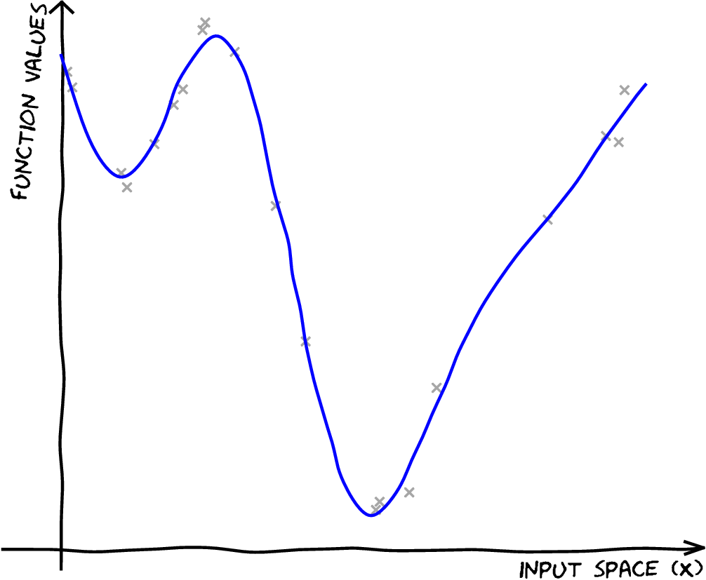
Full Gaussian Process Fit

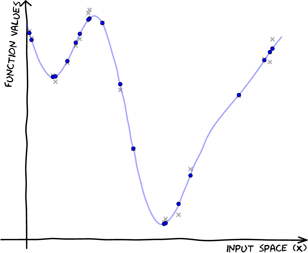
Inducing Variable Fit

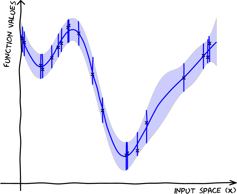
Inducing Variable Param Optimize

Inducing Variable Full Optimize

Eight Optimized Inducing Variables

Full Gaussian Process Fit

Thanks!

References

Álvarez, M.A., Luengo, D., Titsias, M.K., Lawrence, N.D., 2010. Efficient multioutput Gaussian processes through variational inducing kernels. pp. 25–32.

Bui, T.D., Yan, J., Turner, R.E., 2017. A unifying framework for Gaussian process pseudo-point approximations using power expectation propagation. Journal of Machine Learning Research 18, 1–72.

Csató, L., Opper, M., 2002. Sparse on-line Gaussian processes. Neural Computation 14, 641–668.

Dai, Z., Damianou, A., Hensman, J., Lawrence, N.D., 2014. Gaussian process models with parallelization and GPU acceleration.

Damianou, A., 2015. Deep Gaussian processes and variational propagation of uncertainty (PhD thesis). University of Sheffield.

Damianou, A., Lawrence, N.D., 2013. Deep Gaussian processes. pp. 207–215.

Damianou, A., Titsias, M.K., Lawrence, N.D., 2016. Variational inference for latent variables and uncertain inputs in Gaussian processes. Journal of Machine Learning Research 17.

Gal, Y., Wilk, M. van der, Rasmussen, C.E., n.d. Distributed variational inference in sparse Gaussian process regression and latent variable models.

Hensman, J., Fusi, N., Lawrence, N.D., n.d. Gaussian processes for big data.

Hensman, J., Lawrence, N.D., 2014. Nested variational compression in deep Gaussian processes. University of Sheffield.

Hensman, J., Rattray, M., Lawrence, N.D., 2012. Fast variational inference in the conjugate exponential family.

Hoffman, M., Blei, D.M., Wang, C., Paisley, J., 2012. Stochastic variational inference, arXiv preprint arXiv:1206.7051.

King, N.J., Lawrence, N.D., n.d. Fast variational inference for Gaussian Process models through KL-correction. pp. 270–281.

Lawrence, N.D., n.d. Learning for larger datasets with the Gaussian process latent variable model. pp. 243–250.

Lawrence, N.D., Seeger, M., Herbrich, R., n.d. Fast sparse Gaussian process methods: The informative vector machine. pp. 625–632.

Quiñonero Candela, J., Rasmussen, C.E., 2005. A unifying view of sparse approximate Gaussian process regression. Journal of Machine Learning Research 6, 1939–1959.

Salimbeni, H., Deisenroth, M., 2017. Doubly stochastic variational inference for deep Gaussian processes, in: Guyon, I., Luxburg, U.V., Bengio, S., Wallach, H., Fergus, R., Vishwanathan, S., Garnett, R. (Eds.), Advances in Neural Information Processing Systems 30. Curran Associates, Inc., pp. 4591–4602.

Seeger, M.W., Hetzel, A., Dai, Z., Lawrence, N.D., 2017. Auto-differentiating linear algebra. CoRR abs/1710.08717.

Seeger, M., Williams, C.K.I., Lawrence, N.D., n.d. Fast forward selection to speed up sparse Gaussian process regression.

Smola, A.J., Bartlett, P.L., n.d. Sparse greedy Gaussian process regression. pp. 619–625.

Snelson, E., Ghahramani, Z., n.d. Sparse Gaussian processes using pseudo-inputs.

Titsias, M.K., n.d. Variational learning of inducing variables in sparse Gaussian processes. pp. 567–574.

Williams, C.K.I., Seeger, M., n.d. Using the Nyström method to speed up kernel machines. pp. 682–688.

Complexity:	$\mathcal{O}(n^3)$
Storage:	$\mathcal{O}(n^2)$

Complexity:	$\mathcal{O}(nm^2)$
Storage:	$\mathcal{O}(nm)$