Week 12: Deep Gaussian Processes II

[Powerpoint][jupyter][google colab][reveal]

Abstract:

Robot Wireless Data

The robot wireless data is taken from an experiment run by Brian Ferris at University of Washington. It consists of the measurements of WiFi access point signal strengths as Brian walked in a loop. It was published at IJCAI in 2007 (Ferris et al., 2007).

import pods
import numpy as np

data=pods.datasets.robot_wireless()

The ground truth is recorded in the data, the actual loop is given in the plot below.

Robot Wireless Ground Truth

Figure: Ground truth movement for the position taken while recording the multivariate time-course of wireless access point signal strengths.

We will ignore this ground truth in making our predictions, but see if the model can recover something similar in one of the latent layers.

Robot WiFi Data

One challenge with the data is that the signal strength ‘drops out’. This is because the device only tracks a limited number of wifi access points, when one of the access points falls outside the track, the value disappears (in the plot below it reads -0.5). The data is missing, but it is not missing at random because the implication is that the wireless access point must be weak to have dropped from the list of those that are tracked.

Figure: Output dimension 1 from the robot wireless data. This plot shows signal strength changing over time.

Gaussian Process Fit to Robot Wireless Data

Perform a Gaussian process fit on the data using GPy.

m_full = GPy.models.GPRegression(x,yhat)
_ = m_full.optimize() # Optimize parameters of covariance function

Robot WiFi Data GP

Figure: Gaussian process fit to the Robot Wireless dimension 1.

The deep Gaussian process code we are using is research code by Andreas Damianou.

To extend the research code we introduce some approaches to initialization and optimization that we’ll use in examples. These approaches can be found in the deepgp_tutorial.py file.

Deep Gaussian process models also can require some thought in the initialization. Here we choose to start by setting the noise variance to be one percent of the data variance.

import deepgp_tutorial

from deepgp_tutorial import initialize

Secondly, we introduce a staged optimization approach.

Optimization requires moving variational parameters in the hidden layer representing the mean and variance of the expected values in that layer. Since all those values can be scaled up, and this only results in a downscaling in the output of the first GP, and a downscaling of the input length scale to the second GP. It makes sense to first of all fix the scales of the covariance function in each of the GPs.

Sometimes, deep Gaussian processes can find a local minima which involves increasing the noise level of one or more of the GPs. This often occurs because it allows a minimum in the KL divergence term in the lower bound on the likelihood. To avoid this minimum we habitually train with the likelihood variance (the noise on the output of the GP) fixed to some lower value for some iterations.

Next an optimization of the kernel function parameters at each layer is performed, but with the variance of the likelihood fixed. Again, this is to prevent the model minimizing the Kullback-Leibler divergence between the approximate posterior and the prior before achieving a good data-fit.

Finally, all parameters of the model are optimized together.

import deepgp_tutorial

from deepgp_tutorial import staged_optimize

The next code is for visualizing the intermediate layers of the deep model. This visualization is only appropriate for models with intermediate layers containing a single latent variable.

import deepgp_tutorial

from deepgp_tutorial import visualize

The pinball visualization is to bring the pinball-analogy to life in the model. It shows how a ball would fall through the model to end up in the right pbosition. This visualization is only appropriate for models with intermediate layers containing a single latent variable.

import deepgp_tutorial

from deepgp_tutorial import visualize_pinball

The posterior_sample code allows us to see the output sample locations for a given input. This is useful for visualizing the non-Gaussian nature of the output density.

import deepgp_tutorial

from deepgp_tutorial import posterior_sample

Finally, we bind these methods to the DeepGP object for ease of calling.

layers = [y.shape[1], 10, 5, 2, 2, x.shape[1]]
inits = ['PCA']*(len(layers)-1)
kernels = []
for i in layers[1:]:
    kernels += [GPy.kern.RBF(i, ARD=True)]

m = deepgp.DeepGP(layers,Y=y, X=x, inits=inits, 
                  kernels=kernels,
                  num_inducing=50, back_constraint=False)
m.initialize()

m.staged_optimize(messages=(True,True,True))

Robot WiFi Data Deep GP

Figure: Fit of the deep Gaussian process to dimension 1 of the robot wireless data.

Robot WiFi Data Deep GP

Figure: Samples from the deep Gaussian process fit to dimension 1 of the robot wireless data.

Robot WiFi Data Latent Space

Figure: Inferred two dimensional latent space from the model for the robot wireless data.

%pip install gpy

GPy: A Gaussian Process Framework in Python

Gaussian processes are a flexible tool for non-parametric analysis with uncertainty. The GPy software was started in Sheffield to provide a easy to use interface to GPs. One which allowed the user to focus on the modelling rather than the mathematics.

Figure: GPy is a BSD licensed software code base for implementing Gaussian process models in Python. It is designed for teaching and modelling. We welcome contributions which can be made through the GitHub repository https://github.com/SheffieldML/GPy

GPy is a BSD licensed software code base for implementing Gaussian process models in python. This allows GPs to be combined with a wide variety of software libraries.

The software itself is available on GitHub and the team welcomes contributions.

The aim for GPy is to be a probabilistic-style programming language, i.e., you specify the model rather than the algorithm. As well as a large range of covariance functions the software allows for non-Gaussian likelihoods, multivariate outputs, dimensionality reduction and approximations for larger data sets.

The documentation for GPy can be found here.

This notebook depends on PyDeepGP. This library can be installed via pip.

%pip install --upgrade git+https://github.com/SheffieldML/PyDeepGP.git

%pip install mlai

# Late bind setup methods to DeepGP object
from mlai.deepgp_tutorial import initialize
from mlai.deepgp_tutorial import staged_optimize
from mlai.deepgp_tutorial import posterior_sample
from mlai.deepgp_tutorial import visualize
from mlai.deepgp_tutorial import visualize_pinball

import deepgp
deepgp.DeepGP.initialize=initialize
deepgp.DeepGP.staged_optimize=staged_optimize
deepgp.DeepGP.posterior_sample=posterior_sample
deepgp.DeepGP.visualize=visualize
deepgp.DeepGP.visualize_pinball=visualize_pinball

Olympic Marathon Data

Gold medal times for Olympic Marathon since 1896. Marathons before 1924 didn’t have a standardized distance. Present results using pace per km. In 1904 Marathon was badly organized leading to very slow times.

Image from Wikimedia Commons http://bit.ly/16kMKHQ

The first thing we will do is load a standard data set for regression modelling. The data consists of the pace of Olympic Gold Medal Marathon winners for the Olympics from 1896 to present. Let’s load in the data and plot.

%pip install pods

import numpy as np
import pods

data = pods.datasets.olympic_marathon_men()
x = data['X']
y = data['Y']

offset = y.mean()
scale = np.sqrt(y.var())
yhat = (y - offset)/scale

Figure: Olympic marathon pace times since 1896.

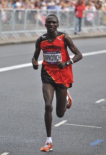
Things to notice about the data include the outlier in 1904, in that year the Olympics was in St Louis, USA. Organizational problems and challenges with dust kicked up by the cars following the race meant that participants got lost, and only very few participants completed. More recent years see more consistently quick marathons.

Alan Turing

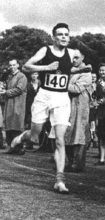
Figure: Alan Turing, in 1946 he was only 11 minutes slower than the winner of the 1948 games. Would he have won a hypothetical games held in 1946? Source: Alan Turing Internet Scrapbook.

If we had to summarise the objectives of machine learning in one word, a very good candidate for that word would be generalization. What is generalization? From a human perspective it might be summarised as the ability to take lessons learned in one domain and apply them to another domain. If we accept the definition given in the first session for machine learning, \[ \text{data} + \text{model} \stackrel{\text{compute}}{\rightarrow} \text{prediction} \] then we see that without a model we can’t generalise: we only have data. Data is fine for answering very specific questions, like “Who won the Olympic Marathon in 2012?”, because we have that answer stored, however, we are not given the answer to many other questions. For example, Alan Turing was a formidable marathon runner, in 1946 he ran a time 2 hours 46 minutes (just under four minutes per kilometer, faster than I and most of the other Endcliffe Park Run runners can do 5 km). What is the probability he would have won an Olympics if one had been held in 1946?

To answer this question we need to generalize, but before we formalize the concept of generalization let’s introduce some formal representation of what it means to generalize in machine learning.

Gaussian Process Fit

Our first objective will be to perform a Gaussian process fit to the data, we’ll do this using the GPy software.

import GPy

m_full = GPy.models.GPRegression(x,yhat)
_ = m_full.optimize() # Optimize parameters of covariance function

The first command sets up the model, then m_full.optimize() optimizes the parameters of the covariance function and the noise level of the model. Once the fit is complete, we’ll try creating some test points, and computing the output of the GP model in terms of the mean and standard deviation of the posterior functions between 1870 and 2030. We plot the mean function and the standard deviation at 200 locations. We can obtain the predictions using y_mean, y_var = m_full.predict(xt)

xt = np.linspace(1870,2030,200)[:,np.newaxis]
yt_mean, yt_var = m_full.predict(xt)
yt_sd=np.sqrt(yt_var)

Now we plot the results using the helper function in mlai.plot.

Figure: Gaussian process fit to the Olympic Marathon data. The error bars are too large, perhaps due to the outlier from 1904.

Fit Quality

In the fit we see that the error bars (coming mainly from the noise variance) are quite large. This is likely due to the outlier point in 1904, ignoring that point we can see that a tighter fit is obtained. To see this make a version of the model, m_clean, where that point is removed.

x_clean=np.vstack((x[0:2, :], x[3:, :]))
y_clean=np.vstack((yhat[0:2, :], yhat[3:, :]))

m_clean = GPy.models.GPRegression(x_clean,y_clean)
_ = m_clean.optimize()

Deep GP Fit

Let’s see if a deep Gaussian process can help here. We will construct a deep Gaussian process with one hidden layer (i.e. one Gaussian process feeding into another).

Build a Deep GP with an additional hidden layer (one dimensional) to fit the model.

import GPy
import deepgp

hidden = 1
m = deepgp.DeepGP([y.shape[1],hidden,x.shape[1]],Y=yhat, X=x, inits=['PCA','PCA'], 
                  kernels=[GPy.kern.RBF(hidden,ARD=True),
                           GPy.kern.RBF(x.shape[1],ARD=True)], # the kernels for each layer
                  num_inducing=50, back_constraint=False)

# Call the initalization
m.initialize()

Now optimize the model.

for layer in m.layers:
    layer.likelihood.variance.constrain_positive(warning=False)
m.optimize(messages=True,max_iters=10000)

m.staged_optimize(messages=(True,True,True))

Olympic Marathon Data Deep GP

Figure: Deep GP fit to the Olympic marathon data. Error bars now change as the prediction evolves.

Olympic Marathon Data Deep GP

Figure: Point samples run through the deep Gaussian process show the distribution of output locations.

Fitted GP for each layer

Now we explore the GPs the model has used to fit each layer. First of all, we look at the hidden layer.

Figure: The mapping from input to the latent layer is broadly, with some flattening as time goes on. Variance is high across the input range.

Figure: The mapping from the latent layer to the output layer.

Olympic Marathon Pinball Plot

Figure: A pinball plot shows the movement of the ‘ball’ as it passes through each layer of the Gaussian processes. Mean directions of movement are shown by lines. Shading gives one standard deviation of movement position. At each layer, the uncertainty is reset. The overal uncertainty is the cumulative uncertainty from all the layers. There is some grouping of later points towards the right in the first layer, which also injects a large amount of uncertainty. Due to flattening of the curve in the second layer towards the right the uncertainty is reduced in final output.

The pinball plot shows the flow of any input ball through the deep Gaussian process. In a pinball plot a series of vertical parallel lines would indicate a purely linear function. For the olypmic marathon data we can see the first layer begins to shift from input towards the right. Note it also does so with some uncertainty (indicated by the shaded backgrounds). The second layer has less uncertainty, but bunches the inputs more strongly to the right. This input layer of uncertainty, followed by a layer that pushes inputs to the right is what gives the heteroschedastic noise.

Gene Expression Example

We now consider an example in gene expression. Gene expression is the measurement of mRNA levels expressed in cells. These mRNA levels show which genes are ‘switched on’ and producing data. In the example we will use a Gaussian process to determine whether a given gene is active, or we are merely observing a noise response.

Della Gatta Gene Data

• Given given expression levels in the form of a time series from Della Gatta et al. (2008).

import numpy as np
import pods

data = pods.datasets.della_gatta_TRP63_gene_expression(data_set='della_gatta',gene_number=937)

x = data['X']
y = data['Y']

offset = y.mean()
scale = np.sqrt(y.var())

Figure: Gene expression levels over time for a gene from data provided by Della Gatta et al. (2008). We would like to understand whether there is signal in the data, or we are only observing noise.

• Want to detect if a gene is expressed or not, fit a GP to each gene Kalaitzis and Lawrence (2011).

Figure: The example is taken from the paper “A Simple Approach to Ranking Differentially Expressed Gene Expression Time Courses through Gaussian Process Regression.” Kalaitzis and Lawrence (2011).

Our first objective will be to perform a Gaussian process fit to the data, we’ll do this using the GPy software.

import GPy

m_full = GPy.models.GPRegression(x,yhat)
m_full.kern.lengthscale=50
_ = m_full.optimize() # Optimize parameters of covariance function

Initialize the length scale parameter (which here actually represents a time scale of the covariance function) to a reasonable value. Default would be 1, but here we set it to 50 minutes, given points are arriving across zero to 250 minutes.

xt = np.linspace(-20,260,200)[:,np.newaxis]
yt_mean, yt_var = m_full.predict(xt)
yt_sd=np.sqrt(yt_var)

Now we plot the results using the helper function in mlai.plot.

Figure: Result of the fit of the Gaussian process model with the time scale parameter initialized to 50 minutes.

Now we try a model initialized with a longer length scale.

m_full2 = GPy.models.GPRegression(x,yhat)
m_full2.kern.lengthscale=2000
_ = m_full2.optimize() # Optimize parameters of covariance function

Figure: Result of the fit of the Gaussian process model with the time scale parameter initialized to 2000 minutes.

Now we try a model initialized with a lower noise.

m_full3 = GPy.models.GPRegression(x,yhat)
m_full3.kern.lengthscale=20
m_full3.likelihood.variance=0.001
_ = m_full3.optimize() # Optimize parameters of covariance function

Figure: Result of the fit of the Gaussian process model with the noise initialized low (standard deviation 0.1) and the time scale parameter initialized to 20 minutes.

Figure:

layers = [y.shape[1], 1,x.shape[1]]
inits = ['PCA']*(len(layers)-1)
kernels = []
for i in layers[1:]:
    kernels += [GPy.kern.RBF(i)]
m = deepgp.DeepGP(layers,Y=yhat, X=x, 
                  inits=inits, 
                  kernels=kernels, # the kernels for each layer
                  num_inducing=20, back_constraint=False)

m.initialize()
m.staged_optimize()

Della Gatta Gene Data Deep GP

Figure: Deep Gaussian process fit to the Della Gatta gene expression data.

Della Gatta Gene Data Deep GP

Figure: Deep Gaussian process samples fitted to the Della Gatta gene expression data.

Della Gatta Gene Data Latent 1

Figure: Gaussian process mapping from input to latent layer for the della Gatta gene expression data.

Della Gatta Gene Data Latent 2

Figure: Gaussian process mapping from latent to output layer for the della Gatta gene expression data.

TP53 Gene Pinball Plot

Figure: A pinball plot shows the movement of the ‘ball’ as it passes through each layer of the Gaussian processes. Mean directions of movement are shown by lines. Shading gives one standard deviation of movement position. At each layer, the uncertainty is reset. The overal uncertainty is the cumulative uncertainty from all the layers. Pinball plot of the della Gatta gene expression data.

Step Function

Next we consider a simple step function data set.

num_low=25
num_high=25
gap = -.1
noise=0.0001
x = np.vstack((np.linspace(-1, -gap/2.0, num_low)[:, np.newaxis],
              np.linspace(gap/2.0, 1, num_high)[:, np.newaxis]))
y = np.vstack((np.zeros((num_low, 1)), np.ones((num_high,1))))
scale = np.sqrt(y.var())
offset = y.mean()
yhat = (y-offset)/scale

Step Function Data

Figure: Simulation study of step function data artificially generated. Here there is a small overlap between the two lines.

Step Function Data GP

We can fit a Gaussian process to the step function data using GPy as follows.

m_full = GPy.models.GPRegression(x,yhat)
_ = m_full.optimize() # Optimize parameters of covariance function

Where GPy.models.GPRegression() gives us a standard GP regression model with exponentiated quadratic covariance function.

The model is optimized using m_full.optimize() which calls an L-BGFS gradient based solver in python.

Figure: Gaussian process fit to the step function data. Note the large error bars and the over-smoothing of the discontinuity. Error bars are shown at two standard deviations.

The resulting fit to the step function data shows some challenges. In particular, the over smoothing at the discontinuity. If we know how many discontinuities there are, we can parameterize them in the step function. But by doing this, we form a semi-parametric model. The parameters indicate how many discontinuities are, and where they are. They can be optimized as part of the model fit. But if new, unforeseen, discontinuities arise when the model is being deployed in practice, these won’t be accounted for in the predictions.

Step Function Data Deep GP

First we initialize a deep Gaussian process with three latent layers (four layers total). Within each layer we create a GP with an exponentiated quadratic covariance (GPy.kern.RBF).

At each layer we use 20 inducing points for the variational approximation.

layers = [y.shape[1], 1, 1, 1,x.shape[1]]
inits = ['PCA']*(len(layers)-1)
kernels = []
for i in layers[1:]:
    kernels += [GPy.kern.RBF(i)]
    
m = deepgp.DeepGP(layers,Y=yhat, X=x, 
                  inits=inits, 
                  kernels=kernels, # the kernels for each layer
                  num_inducing=20, back_constraint=False)

Once the model is constructed we initialize the parameters, and perform the staged optimization which starts by optimizing variational parameters with a low noise and proceeds to optimize the whole model.

m.initialize()
m.staged_optimize()

We plot the output of the deep Gaussian process fitted to the step data as follows.

The deep Gaussian process does a much better job of fitting the data. It handles the discontinuity easily, and error bars drop to smaller values in the regions of data.

Figure: Deep Gaussian process fit to the step function data.

Step Function Data Deep GP

The samples of the model can be plotted with the helper function from mlai.plot, model_sample

The samples from the model show that the error bars, which are informative for Gaussian outputs, are less informative for this model. They make clear that the data points lie, in output mainly at 0 or 1, or occasionally in between.

Figure: Samples from the deep Gaussian process model for the step function fit.

The visualize code allows us to inspect the intermediate layers in the deep GP model to understand how it has reconstructed the step function.

Figure: From top to bottom, the Gaussian process mapping function that makes up each layer of the resulting deep Gaussian process.

A pinball plot can be created for the resulting model to understand how the input is being translated to the output across the different layers.

Figure: Pinball plot of the deep GP fitted to the step function data. Each layer of the model pushes the ‘ball’ towards the left or right, saturating at 1 and 0. This causes the final density to be be peaked at 0 and 1. Transitions occur driven by the uncertainty of the mapping in each layer.

import pods

data = pods.datasets.mcycle()
x = data['X']
y = data['Y']
scale=np.sqrt(y.var())
offset=y.mean()
yhat = (y - offset)/scale

Motorcycle Helmet Data

Figure: Motorcycle helmet data. The data consists of acceleration readings on a motorcycle helmet undergoing a collision. The data exhibits heteroschedastic (time varying) noise levles and non-stationarity.

m_full = GPy.models.GPRegression(x,yhat)
_ = m_full.optimize() # Optimize parameters of covariance function

Motorcycle Helmet Data GP

Figure: Gaussian process fit to the motorcycle helmet accelerometer data.

Motorcycle Helmet Data Deep GP

import deepgp

layers = [y.shape[1], 1, x.shape[1]]
inits = ['PCA']*(len(layers)-1)
kernels = []
for i in layers[1:]:
    kernels += [GPy.kern.RBF(i)]
m = deepgp.DeepGP(layers,Y=yhat, X=x, 
                  inits=inits, 
                  kernels=kernels, # the kernels for each layer
                  num_inducing=20, back_constraint=False)



m.initialize()

m.staged_optimize(iters=(1000,1000,10000), messages=(True, True, True))

Figure: Deep Gaussian process fit to the motorcycle helmet accelerometer data.

Motorcycle Helmet Data Deep GP

Figure: Samples from the deep Gaussian process as fitted to the motorcycle helmet accelerometer data.

Motorcycle Helmet Data Latent 1

Figure: Mappings from the input to the latent layer for the motorcycle helmet accelerometer data.

Motorcycle Helmet Data Latent 2

Figure: Mappings from the latent layer to the output layer for the motorcycle helmet accelerometer data.

Motorcycle Helmet Pinball Plot

Figure: Pinball plot for the mapping from input to output layer for the motorcycle helmet accelerometer data.

‘High Five’ Motion Capture Data

Motion capture data from the CMU motion capture data base (CMU Motion Capture Lab, 2003). It contains two subjects approaching each other and executing a ‘high five’. The subjects are number 10 and 11 and their motion numbers are 21.

import pods

data = pods.datasets.cmu_mocap_high_five()

The data dictionary contains the keys ‘Y1’ and ‘Y2’, which represent the motions of the two different subjects. Their skeleton files are included in the keys ‘skel1’ and ‘skel2’.

data['Y1'].shape
data['Y2'].shape

The data was used in the hierarchical GP-LVM paper (Lawrence and Moore, 2007) in an experiment that was also recreated in the Deep Gaussian process paper (Damianou and Lawrence, 2013).

print(data['citation'])

And extra information about the data is included, as standard, under the keys info and details.

print(data['info'])
print()
print(data['details'])

Shared LVM

Figure: Shared latent variable model structure. Here two related data sets are brought together with a set of latent variables that are partially shared and partially specific to one of the data sets.

Figure: Latent spaces of the ‘high five’ data. The structure of the model is automatically learnt. One of the latent spaces is coordinating how the two figures walk together, the other latent spaces contain latent variables that are specific to each of the figures separately.

Subsample of the MNIST Data

We will look at a sub-sample of the MNIST digit data set.

First load in the MNIST data set from scikit learn. This can take a little while because it’s large to download.

from sklearn.datasets import fetch_openml

mnist = fetch_openml('mnist_784')

Sub-sample the dataset to make the training faster.

import numpy as np

np.random.seed(0)
digits = [0,1,2,3,4]
N_per_digit = 100
Y = []
labels = []
for d in digits:
    imgs = mnist['data'][mnist['target']==str(d)]
    Y.append(imgs.loc[np.random.permutation(imgs.index)[:N_per_digit]])
    labels.append(np.ones(N_per_digit)*d)
Y = np.vstack(Y).astype(np.float64)
labels = np.hstack(labels)
Y /= 255

Fitting a Deep GP to a the MNIST Digits Subsample

We now look at the deep Gaussian processes’ capacity to perform unsupervised learning.

Fit a Deep GP

We’re going to fit a Deep Gaussian process model to the MNIST data with two hidden layers. Each of the two Gaussian processes (one from the first hidden layer to the second, one from the second hidden layer to the data) has an exponentiated quadratic covariance.

import deepgp
import GPy

num_latent = 2
num_hidden_2 = 5
m = deepgp.DeepGP([Y.shape[1],num_hidden_2,num_latent],
                  Y,
                  kernels=[GPy.kern.RBF(num_hidden_2,ARD=True), 
                           GPy.kern.RBF(num_latent,ARD=False)], 
                  num_inducing=50, back_constraint=False, 
                  encoder_dims=[[200],[200]])

Initialization

Just like deep neural networks, there are some tricks to intitializing these models. The tricks we use here include some early training of the model with model parameters constrained. This gives the variational inducing parameters some scope to tighten the bound for the case where the noise variance is small and the variances of the Gaussian processes are around 1.

m.obslayer.likelihood.variance[:] = Y.var()*0.01
for layer in m.layers:
    layer.kern.variance.fix(warning=False)
    layer.likelihood.variance.fix(warning=False)

We now we optimize for a hundred iterations with the constrained model.

m.optimize(messages=False,max_iters=100)

Now we remove the fixed constraint on the kernel variance parameters, but keep the noise output constrained, and run for a further 100 iterations.

for layer in m.layers:
    layer.kern.variance.constrain_positive(warning=False)
m.optimize(messages=False,max_iters=100)

Finally we unconstrain the layer likelihoods and allow the full model to be trained for 1000 iterations.

for layer in m.layers:
    layer.likelihood.variance.constrain_positive(warning=False)
m.optimize(messages=True,max_iters=10000)

Visualize the latent space of the top layer

Now the model is trained, let’s plot the mean of the posterior distributions in the top latent layer of the model.

Figure: Latent space for the deep Gaussian process learned through unsupervised learning and fitted to a subset of the MNIST digits subsample.

Visualize the latent space of the intermediate layer

We can also visualize dimensions of the intermediate layer. First the lengthscale of those dimensions is given by

m.obslayer.kern.lengthscale

Figure: Visualisation of the intermediate layer, plot of dimension 1 vs dimension 0.

Figure: Visualisation of the intermediate layer, plot of dimension 1 vs dimension 0.

Figure: Visualisation of the intermediate layer, plot of dimension 1 vs dimension 0.

Figure: Visualisation of the intermediate layer, plot of dimension 1 vs dimension 0.

Generate From Model

Now we can take a look at a sample from the model, by drawing a Gaussian random sample in the latent space and propagating it through the model.

rows = 10
cols = 20
t=np.linspace(-1, 1, rows*cols)[:, None]
kern = GPy.kern.RBF(1,lengthscale=0.05)
cov = kern.K(t, t)
x = np.random.multivariate_normal(np.zeros(rows*cols), cov, num_latent).T

Figure: These digits are produced by taking a tour of the two dimensional latent space (as described by a Gaussian process sample) and mapping the tour into the data space. We visualize the mean of the mapping in the images.

Deep Health

Figure: The deep health model uses different layers of abstraction in the deep Gaussian process to represent information about diagnostics and treatment to model interelationships between a patients different data modalities.

From a machine learning perspective, we’d like to be able to interrelate all the different modalities that are informative about the state of the disease. For deep health, the notion is that the state of the disease is appearing at the more abstract levels, as we descend the model, we express relationships between the more abstract concept, that sits within the physician’s mind, and the data we can measure.

Thanks!

For more information on these subjects and more you might want to check the following resources.

• twitter: @lawrennd
• podcast: The Talking Machines
• newspaper: Guardian Profile Page
• blog: http://inverseprobability.com

References