Week 7: Non Gaussian Likelihoods

[Powerpoint][jupyter][google colab][reveal]

Abstract:

%pip install gpy

GPy: A Gaussian Process Framework in Python

Gaussian processes are a flexible tool for non-parametric analysis with uncertainty. The GPy software was started in Sheffield to provide a easy to use interface to GPs. One which allowed the user to focus on the modelling rather than the mathematics.

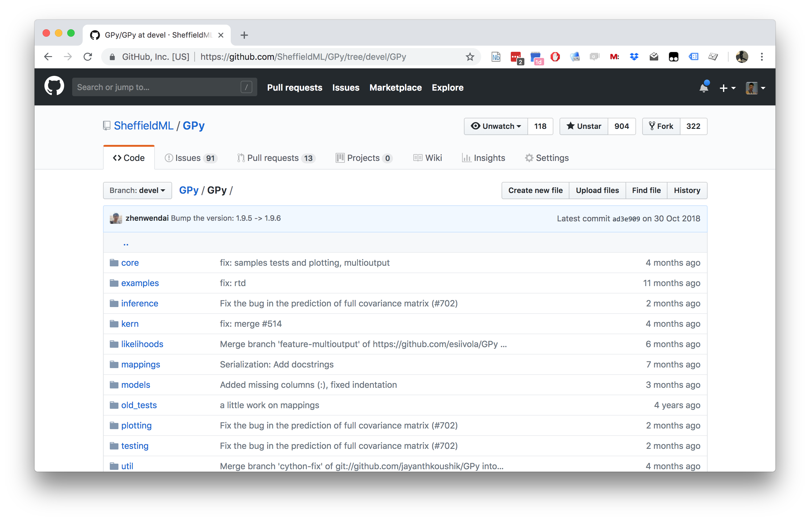
Figure: GPy is a BSD licensed software code base for implementing Gaussian process models in Python. It is designed for teaching and modelling. We welcome contributions which can be made through the GitHub repository https://github.com/SheffieldML/GPy

GPy is a BSD licensed software code base for implementing Gaussian process models in python. This allows GPs to be combined with a wide variety of software libraries.

The software itself is available on GitHub and the team welcomes contributions.

The aim for GPy is to be a probabilistic-style programming language, i.e., you specify the model rather than the algorithm. As well as a large range of covariance functions the software allows for non-Gaussian likelihoods, multivariate outputs, dimensionality reduction and approximations for larger data sets.

The documentation for GPy can be found here.

Non Gaussian Likelihoods

[Gaussian processes model functions. If our observation is a corrupted version of this function and the corruption process is also Gaussian, it is trivial to account for this. However, there are many circumstances where our observation may be non Gaussian. In these cases we need to turn to approximate inference techniques. As a simple illustration, we’ll use a dataset of binary observations of the language that is spoken in different regions of East-Timor. First we will load the data and a couple of libraries to visualize it.}

from matplotlib.patches import Polygon
from matplotlib.collections import PatchCollection
import cPickle as pickle
import urllib

urllib.urlretrieve('http://staffwww.dcs.sheffield.ac.uk/people/M.Zwiessele/gpss/lab2/EastTimor.pickle', 'EastTimor2.pickle')

# Load the data
with open("./EastTimor2.pickle","rb") as f:
    X,y,polygons = pickle.load(f)

Now we will create a map of East Timor and, using GPy, plot the data on top of it. A classification model can be defined in a similar way to the regression model, but now using GPy.models.GPClassification. However, once we’ve define the model, we also need to update the approximation to the likelihood. This runs the Expectation propagation updates.

import GPy

#Define the model
kern = GPy.kern.RBF(2)
m = GPy.models.GPClassification(X,y, kernel=kern)
print(m)

The decision boundary should be quite poor! However we haven’t optimized the model. Try the following:

m.optimize()
print(m)

The optimization is based on the likelihood approximation that was made after we constructed the model. However, because we’ve now changed the model parameters the quality of that approximation has now probably deteriorated. To improve the model we should iterate between updating the Expectation propagation approximation and optimizing the model parameters.

Olympic Marathon Data

Gold medal times for Olympic Marathon since 1896. Marathons before 1924 didn’t have a standardized distance. Present results using pace per km. In 1904 Marathon was badly organized leading to very slow times.

Image from Wikimedia Commons http://bit.ly/16kMKHQ

The first thing we will do is load a standard data set for regression modelling. The data consists of the pace of Olympic Gold Medal Marathon winners for the Olympics from 1896 to present. Let’s load in the data and plot.

%pip install pods

import numpy as np
import pods

data = pods.datasets.olympic_marathon_men()
x = data['X']
y = data['Y']

offset = y.mean()
scale = np.sqrt(y.var())
yhat = (y - offset)/scale

Figure: Olympic marathon pace times since 1896.

Things to notice about the data include the outlier in 1904, in that year the Olympics was in St Louis, USA. Organizational problems and challenges with dust kicked up by the cars following the race meant that participants got lost, and only very few participants completed. More recent years see more consistently quick marathons.

Alan Turing

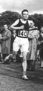
Figure: Alan Turing, in 1946 he was only 11 minutes slower than the winner of the 1948 games. Would he have won a hypothetical games held in 1946? Source: Alan Turing Internet Scrapbook.

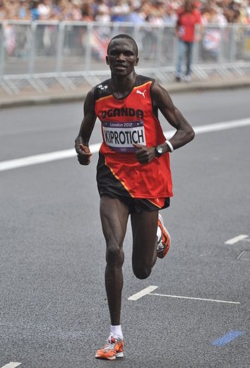
If we had to summarise the objectives of machine learning in one word, a very good candidate for that word would be generalization. What is generalization? From a human perspective it might be summarised as the ability to take lessons learned in one domain and apply them to another domain. If we accept the definition given in the first session for machine learning, \[ \text{data} + \text{model} \stackrel{\text{compute}}{\rightarrow} \text{prediction} \] then we see that without a model we can’t generalise: we only have data. Data is fine for answering very specific questions, like “Who won the Olympic Marathon in 2012?”, because we have that answer stored, however, we are not given the answer to many other questions. For example, Alan Turing was a formidable marathon runner, in 1946 he ran a time 2 hours 46 minutes (just under four minutes per kilometer, faster than I and most of the other Endcliffe Park Run runners can do 5 km). What is the probability he would have won an Olympics if one had been held in 1946?

To answer this question we need to generalize, but before we formalize the concept of generalization let’s introduce some formal representation of what it means to generalize in machine learning.

Gaussian Process Fit

Our first objective will be to perform a Gaussian process fit to the data, we’ll do this using the GPy software.

import GPy

m_full = GPy.models.GPRegression(x,yhat)
_ = m_full.optimize() # Optimize parameters of covariance function

The first command sets up the model, then m_full.optimize() optimizes the parameters of the covariance function and the noise level of the model. Once the fit is complete, we’ll try creating some test points, and computing the output of the GP model in terms of the mean and standard deviation of the posterior functions between 1870 and 2030. We plot the mean function and the standard deviation at 200 locations. We can obtain the predictions using y_mean, y_var = m_full.predict(xt)

xt = np.linspace(1870,2030,200)[:,np.newaxis]
yt_mean, yt_var = m_full.predict(xt)
yt_sd=np.sqrt(yt_var)

Now we plot the results using the helper function in mlai.plot.

Figure: Gaussian process fit to the Olympic Marathon data. The error bars are too large, perhaps due to the outlier from 1904.

Fit Quality

In the fit we see that the error bars (coming mainly from the noise variance) are quite large. This is likely due to the outlier point in 1904, ignoring that point we can see that a tighter fit is obtained. To see this make a version of the model, m_clean, where that point is removed.

x_clean=np.vstack((x[0:2, :], x[3:, :]))
y_clean=np.vstack((yhat[0:2, :], yhat[3:, :]))

m_clean = GPy.models.GPRegression(x_clean,y_clean)
_ = m_clean.optimize()

Robust Regression: A Running Example

We already considered the olympic marathon data. In 1904 we noted there was an outlier example. Today we’ll see if we can deal with that outlier by considering a non-Gaussian likelihood. Noise sampled from a Student-\(t\) density is heavier tailed than that sampled from a Gaussian. However, it cannot be trivially assimilated into the Gaussian process. Below we use the Laplace approximation to incorporate this noise model.

GPy.likelihoods.StudentT?

# make a student t likelihood with standard parameters
t_distribution = GPy.likelihoods.StudentT(deg_free=3, sigma2=2)
laplace = GPy.inference.latent_function_inference.Laplace()

kern = GPy.kern.RBF(1, lengthscale=5) + GPy.kern.Bias(1)
model = GPy.core.GP(x, y, kernel=kern, inference_method=laplace, likelihood=t_distribution)
model.constrain_positive('t_noise')

model.optimize(messages=True)
display(model)

Figure: Fit to the Olympic marathon data using the Student-\(t\) likelihood and the Laplace approximation.

Sparse GP Classification

In this section we’ll combine expectation propagation with the low rank approximation to build a simple image classification application. For this toy example we’ll classify whether or not the subject of the image is wearing glasses.

Correspond to whether the subject of the image is wearing glasses. Set up the ipython environment and download the data:

from scipy import io

First let’s retrieve some data. We will use the ORL faces data set, our objective will be to classify whether or not the subject in an image is wearing glasess.

Here’s a simple way to visualise the data. Each pixel in the image will become an input to the GP.

import pods

data = pods.datasets.olivetti_glasses()
X = data['X']
y = data['Y']
Xtest = data['Xtest']
ytest = data['Ytest']
print(data['info'], data['details'], data['citation'])

Figure: Image from the Oivetti glasses data sets.

Next we choose some inducing inputs. Here we’ve chosen inducing inputs by applying k-means clustering to the training data. Think about whether this is a good scheme for choosing the inputs? Can you devise a better one?

X.shape
y.shape
print(X)

from scipy import cluster

M = 8
X = (X - X.mean(0)[np.newaxis,:])/X.std(0)[np.newaxis,:]
Z = np.random.permutation(X)[:M]

Finally, we’re ready to build the classifier object.

kern = GPy.kern.RBF(X.shape[1],lengthscale=20) + GPy.kern.White(X.shape[1],0.001)
model = GPy.models.SparseGPClassification(X, y, kernel=kern, Z=Z)
model.optimize(messages=True)
display(model)

Figure: The gradients of the inducing variable.

Thanks!

For more information on these subjects and more you might want to check the following resources.

• twitter: @lawrennd
• podcast: The Talking Machines
• newspaper: Guardian Profile Page
• blog: http://inverseprobability.com

References