Week 5: Multi-output Gaussian Processes

[Powerpoint][jupyter][google colab][reveal]

Abstract:

In this lecture we review multi-output Gaussian processes. Introducing them initially through a Kalman filter representation of a GP.

%pip install gpy

GPy: A Gaussian Process Framework in Python

Gaussian processes are a flexible tool for non-parametric analysis with uncertainty. The GPy software was started in Sheffield to provide a easy to use interface to GPs. One which allowed the user to focus on the modelling rather than the mathematics.

Figure: GPy is a BSD licensed software code base for implementing Gaussian process models in Python. It is designed for teaching and modelling. We welcome contributions which can be made through the GitHub repository https://github.com/SheffieldML/GPy

GPy is a BSD licensed software code base for implementing Gaussian process models in python. This allows GPs to be combined with a wide variety of software libraries.

The software itself is available on GitHub and the team welcomes contributions.

The aim for GPy is to be a probabilistic-style programming language, i.e., you specify the model rather than the algorithm. As well as a large range of covariance functions the software allows for non-Gaussian likelihoods, multivariate outputs, dimensionality reduction and approximations for larger data sets.

The documentation for GPy can be found here.

Simple Kalman Filter

• We have state vector \(\mathbf{X}= \left[\mathbf{ x}_1 \dots \mathbf{ x}_q\right] \in \mathbb{R}^{T \times q}\) and if each state evolves independently we have \[ \begin{align*} p(\mathbf{X}) &= \prod_{i=1}^qp(\mathbf{ x}_{:, i}) \\ p(\mathbf{ x}_{:, i}) &= \mathcal{N}\left(\mathbf{ x}_{:, i}|\mathbf{0},\mathbf{K}\right). \end{align*} \]

• We want to obtain outputs through: \[ \mathbf{ y}_{i, :} = \mathbf{W}\mathbf{ x}_{i, :} \]

Stacking and Kronecker Products

• Represent with a ‘stacked’ system: \[ p(\mathbf{ x}) = \mathcal{N}\left(\mathbf{ x}|\mathbf{0},\mathbf{I}\otimes \mathbf{K}\right) \] where the stacking is placing each column of \(\mathbf{X}\) one on top of another as \[ \mathbf{ x}= \begin{bmatrix} \mathbf{ x}_{:, 1}\\ \mathbf{ x}_{:, 2}\\ \vdots\\ \mathbf{ x}_{:, q} \end{bmatrix} \]

Kronecker Product

Figure: Illustration of the Kronecker product.

Figure: Kronecker product between two matrices.

Stacking and Kronecker Products

• Represent with a ‘stacked’ system: \[p (\mathbf{ x}) = \mathcal{N}\left(\mathbf{ x}|\mathbf{0},\mathbf{I}\otimes \mathbf{K}\right) \] where the stacking is placing each column of \(\mathbf{X}\) one on top of another as \[ \mathbf{ x}= \begin{bmatrix} \mathbf{ x}_{:, 1}\\ \mathbf{ x}_{:, 2}\\ \vdots\\ \mathbf{ x}_{:, q} \end{bmatrix} \]

Column Stacking

For this stacking the marginal distribution over time is given by the block diagonals.

Figure: The marginal distribution for the first three variables (highlighted) is givne by \(\mathbf{K}\) when the form of stacking is \(\mathbf{I}\otimes \mathbf{K}\). This is the ‘column stacking’ case.

Two Ways of Stacking

Can also stack each row of \(\mathbf{X}\) to form column vector: \[\mathbf{ x}= \begin{bmatrix} \mathbf{ x}_{1, :}\\ \mathbf{ x}_{2, :}\\ \vdots\\ \mathbf{ x}_{T, :} \end{bmatrix}\] \[p(\mathbf{ x}) = \mathcal{N}\left(\mathbf{ x}|\mathbf{0},\mathbf{K}\otimes \mathbf{I}\right)\]

Row Stacking

For this stacking the marginal distribution over the latent dimensions is given by the block diagonals.

Figure: The marginal distribution for the first three variables (highlighted) is independent when the form of stacking is \(\mathbf{K}\otimes \mathbf{I}\). This is the ‘row stacking’ case.

Mapping from Latent Process to Observed

Figure: Mapping from latent process to observed

Observed Process

The observations are related to the latent points by a linear mapping matrix, \[ \mathbf{ y}_{i, :} = \mathbf{W}\mathbf{ x}_{i, :} + \boldsymbol{ \epsilon}_{i, :} \] \[ \boldsymbol{ \epsilon}\sim \mathcal{N}\left(\mathbf{0},\sigma^2\mathbf{I}\right) \]

Figure:

Output Covariance

This leads to a covariance of the form \[ (\mathbf{I}\otimes \mathbf{W}) (\mathbf{K}\otimes \mathbf{I}) (\mathbf{I}\otimes \mathbf{W}^\top) + \mathbf{I}\sigma^2 \] Using \((\mathbf{A}\otimes\mathbf{B}) (\mathbf{C}\otimes\mathbf{D}) = \mathbf{A}\mathbf{C} \otimes \mathbf{B}\mathbf{D}\) This leads to \[ \mathbf{K}\otimes {\mathbf{W}}{\mathbf{W}}^\top + \mathbf{I}\sigma^2 \] or \[ \mathbf{ y}\sim \mathcal{N}\left(\mathbf{0},\mathbf{W}\mathbf{W}^\top \otimes \mathbf{K}+ \mathbf{I}\sigma^2\right) \]

Kernels for Vector Valued Outputs: A Review

Kronecker Structure GPs

• This Kronecker structure leads to several published models. \[ (\mathbf{K}(\mathbf{ x},\mathbf{ x}^\prime))_{i,i^\prime}=k(\mathbf{ x},\mathbf{ x}^\prime)k_T(i,i^\prime), \] where \(k\) has \(\mathbf{ x}\) and \(k_T\) has \(n\) as inputs.

• Can think of multiple output covariance functions as covariances with augmented input.

• Alongside \(\mathbf{ x}\) we also input the \(i\) associated with the output of interest.

Separable Covariance Functions

• Taking \(\mathbf{B}= {\mathbf{W}}{\mathbf{W}}^\top\) we have a matrix expression across outputs. \[\mathbf{K}(\mathbf{ x},\mathbf{ x}^\prime)=k(\mathbf{ x},\mathbf{ x}^\prime)\mathbf{B},\] where \(\mathbf{B}\) is a \(p\times p\) symmetric and positive semi-definite matrix.

• \(\mathbf{B}\) is called the coregionalization matrix.

• We call this class of covariance functions separable due to their product structure.

Sum of Separable Covariance Functions

• In the same spirit a more general class of kernels is given by \[\mathbf{K}(\mathbf{ x},\mathbf{ x}^\prime)=\sum_{j=1}^qk_{j}(\mathbf{ x},\mathbf{ x}^\prime)\mathbf{B}_{j}.\]

• This can also be written as \[\mathbf{K}(\mathbf{X}, \mathbf{X}) = \sum_{j=1}^q\mathbf{B}_{j}\otimes k_{j}(\mathbf{X}, \mathbf{X}),\]

• This is like several Kalman filter-type models added together, but each one with a different set of latent functions.

• We call this class of kernels sum of separable kernels (SoS kernels).

Geostatistics

• Use of GPs in Geostatistics is called kriging.

• These multi-output GPs pioneered in geostatistics: prediction over vector-valued output data is known as cokriging.

• The model in geostatistics is known as the linear model of coregionalization (LMC, Journel and Huijbregts (1978) Goovaerts (1997)).

• Most machine learning multitask models can be placed in the context of the LMC model.

Weighted sum of Latent Functions

• In the linear model of coregionalization (LMC) outputs are expressed as linear combinations of independent random functions.

• In the LMC, each component \(f_i\) is expressed as a linear sum \[f_i(\mathbf{ x}) = \sum_{j=1}^q{w}_{i,{j}}{u}_{j}(\mathbf{ x}).\] where the latent functions are independent and have covariance functions \(k_{j}(\mathbf{ x},\mathbf{ x}^\prime)\).

• The processes \(\{f_j(\mathbf{ x})\}_{j=1}^q\) are independent for \(q\neq {j}^\prime\).

Kalman Filter Special Case

• The Kalman filter is an example of the LMC where \({u}_i(\mathbf{ x}) \rightarrow {x}_i(t)\).

• I.e. we’ve moved form time input to a more general input space.

• In matrix notation:

  1. Kalman filter \[\mathbf{F}= {\mathbf{W}}\mathbf{X}\]
  2. LMC \[\mathbf{F}= {\mathbf{W}}{\mathbf{U}}\] where the rows of these matrices \({\mathbf{F}}\), \(\mathbf{X}\), \({\mathbf{U}}\) each contain \(q\) samples from their corresponding functions at a different time (Kalman filter) or spatial location (LMC).

Intrinsic Coregionalization Model

• If one covariance used for latent functions (like in Kalman filter).

• This is called the intrinsic coregionalization model (ICM, Goovaerts (1997)).

• The kernel matrix corresponding to a dataset \(\mathbf{X}\) takes the form \[ \mathbf{K}(\mathbf{X}, \mathbf{X}) = \mathbf{B}\otimes k(\mathbf{X}, \mathbf{X}). \]

Autokrigeability

• If outputs are noise-free, maximum likelihood is equivalent to independent fits of \(\mathbf{B}\) and \(k(\mathbf{ x}, \mathbf{ x}^\prime)\) (Helterbrand and Cressie, 1994).

• In geostatistics this is known as autokrigeability (Wackernagel, 2003).

• In multitask learning its the cancellation of intertask transfer (Bonilla et al., n.d.).

Intrinsic Coregionalization Model

\[ \mathbf{K}(\mathbf{X}, \mathbf{X}) = \mathbf{ w}\mathbf{ w}^\top \otimes k(\mathbf{X}, \mathbf{X}). \]

\[ \mathbf{ w}= \begin{bmatrix} 1 \\ 5\end{bmatrix} \] \[ \mathbf{B}= \begin{bmatrix} 1 & 5\\ 5&25\end{bmatrix} \]

Intrinsic Coregionalization Model Covariance

import mlai

from mlai import icm_cov

Figure: Intrinsic coregionalization model covariance function.

Intrinsic Coregionalization Model

\[ \mathbf{K}(\mathbf{X}, \mathbf{X}) = \mathbf{B}\otimes k(\mathbf{X}, \mathbf{X}). \]

\[ \mathbf{B}= \begin{bmatrix} 1 & 0.5\\ 0.5& 1.5\end{bmatrix} \]

LMC Samples

\[\mathbf{K}(\mathbf{X}, \mathbf{X}) = \mathbf{B}_1 \otimes k_1(\mathbf{X}, \mathbf{X}) + \mathbf{B}_2 \otimes k_2(\mathbf{X}, \mathbf{X})\]

\[\mathbf{B}_1 = \begin{bmatrix} 1.4 & 0.5\\ 0.5& 1.2\end{bmatrix}\] \[{\ell}_1 = 1\] \[\mathbf{B}_2 = \begin{bmatrix} 1 & 0.5\\ 0.5& 1.3\end{bmatrix}\] \[{\ell}_2 = 0.2\]

LMC in Machine Learning and Statistics

• Used in machine learning for GPs for multivariate regression and in statistics for computer emulation of expensive multivariate computer codes.

• Imposes the correlation of the outputs explicitly through the set of coregionalization matrices.

• Setting \(\mathbf{B}= \mathbf{I}_p\) assumes outputs are conditionally independent given the parameters \(\boldsymbol{ \theta}\). (Lawrence and Platt, 2004; Minka and Picard, 1997; Yu et al., 2005).

• More recent approaches for multiple output modeling are different versions of the linear model of coregionalization.

Semiparametric Latent Factor Model

• Coregionalization matrices are rank 1 Teh et al. (n.d.). rewrite equation as \[\mathbf{K}(\mathbf{X}, \mathbf{X}) = \sum_{j=1}^q\mathbf{ w}_{:, {j}}\mathbf{ w}^{\top}_{:, {j}} \otimes k_{j}(\mathbf{X}, \mathbf{X}).\]

• Like the Kalman filter, but each latent function has a different covariance.

• Authors suggest using an exponentiated quadratic characteristic length-scale for each input dimension.

Semi Parametric Latent Factor Covariance

import mlai

from mlai import icm_cov

import mlai

from mlai import slfm_cov

import mlai.plot as plot
import mlai
import numpy as np

K, anim=plot.animate_covariance_function(mlai.compute_kernel, 
                                         kernel=slfm_cov, subkernel=eq_cov,
                                         W = np.asarray([[1],[5]])

from IPython.core.display import HTML

Semiparametric Latent Factor Model Samples

\[ \mathbf{K}(\mathbf{X}, \mathbf{X}) = \mathbf{ w}_{:, 1}\mathbf{ w}_{:, 1}^\top \otimes k_1(\mathbf{X}, \mathbf{X}) + \mathbf{ w}_{:, 2} \mathbf{ w}_{:, 2}^\top \otimes k_2(\mathbf{X}, \mathbf{X}) \]

\[ \mathbf{ w}_1 = \begin{bmatrix} 0.5 \\ 1\end{bmatrix} \] \[ \mathbf{ w}_2 = \begin{bmatrix} 1 \\ 0.5\end{bmatrix} \]

Gaussian processes for Multi-task, Multi-output and Multi-class

• Bonilla et al. (n.d.) suggest ICM for multitask learning.

• Use a PPCA form for \(\mathbf{B}\): similar to our Kalman filter example.

• Refer to the autokrigeability effect as the cancellation of inter-task transfer.

• Also discuss the similarities between the multi-task GP and the ICM, and its relationship to the SLFM and the LMC.

Multitask Classification

• Mostly restricted to the case where the outputs are conditionally independent given the hyperparameters \(\boldsymbol{\phi}\) (Lawrence and Platt, 2004; Minka and Picard, 1997; Rasmussen and Williams, 2006; Seeger and Jordan, 2004; Williams and Barber, 1998; Yu et al., 2005).

• Intrinsic coregionalization model has been used in the multiclass scenario. Skolidis and Sanguinetti (2011) use the intrinsic coregionalization model for classification, by introducing a probit noise model as the likelihood.

• Posterior distribution is no longer analytically tractable: approximate inference is required.

Computer Emulation

• A statistical model used as a surrogate for a computationally expensive computer model.

• Higdon et al. (2008) use the linear model of coregionalization to model images representing the evolution of the implosion of steel cylinders.

• In Conti and O’Hagan (2009) use the ICM to model a vegetation model: called the Sheffield Dynamic Global Vegetation Model Woodward et al. (1998).

Modelling Multiple Outputs

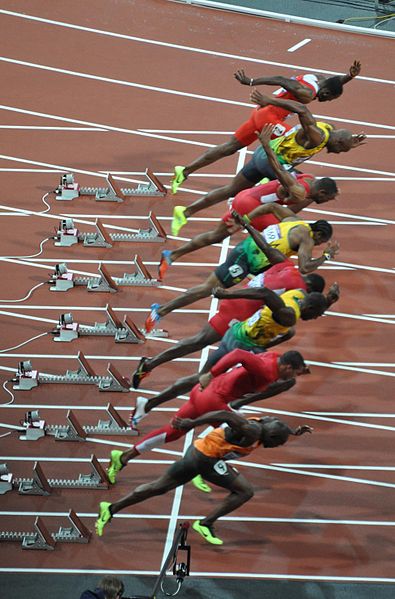
Running Example

Olympic Sprint Data

Gold medal times for Olympic Sprints for Men and Women 100m, 200m, 400m In early years of olympics not all events run.

Image from Wikimedia Commons http://bit.ly/16kMKHQ by Darren Wilkinson

%pip install pods

The first think we will look at is a multiple output model. Our aim is to jointly model all sprinting events from olympics since 1896. Data is provided by Rogers & Girolami’s “First Course in Machine Learning”. Firstly, let’s load in the data.

import pods
import numpy as np

data = pods.datasets.olympic_sprints()
X = data['X']
y = data['Y']
print(data['info'], data['details'])

When using data sets it’s good practice to cite the originators of the data, you can get information about the source of the data from data['citation']

print(data['citation'])

The data consists of all the male and female sprinting data for 100m, 200m and 400m since 1896 (six outputs in total). The output information can be found from: data['output_info']

print(data['output_info'])

In GPy we deal with multiple output data in a particular way. We specify the output we are interested in for modelling as an additional input. So whilst for this data, normally, the only input would be the year of the event. We additionally have an input giving the index of the output we are modelling. This can be seen from examining data['X'].

print('First column of X contains the olympic years.')
print(data['X'][:, 0])
print('Second column of X contains the event index.')
print(data['X'][:, 1])

Now let’s plot the data

Figure: Olympic sprint gold medal winning times from Rogers and Girolami (2011).

In the plot above red is women’s events, blue is men’s. Squares are 400 m, crosses 200m and circles 100m. Not all events were run in all years, for example the women’s 400 m only started in 1964.

Gaussian Process Fit

We will perform a multi-output Gaussian process fit to the data, we’ll do this using the GPy software.

We will look at modelling the data using coregionalization approaches described in this morning’s lecture. We introduced these approaches through the Kronecker product. To indicate we want to construct a covariance function of this type in GPy we’ve overloaded the ** operator. Stricly speaking this operator means to the power of (like ^ in MATLAB). But for covariance functions we’ve used it to indicate a tensor product. The linear models of coregionalization we introduced in the lecture were all based on combining a matrix with a standard covariance function. We can think of the matrix as a particular type of covariance function, whose elements are referenced using the event indices. I.e. \(k(0, 0)\) references the first row and column of the coregionalization matrix. \(k(1, 0)\) references the second row and first column of the coregionalization matrix. Under this set up, we want to build a covariance where the first column from the features (the years) is passed to a covariance function, and the second column from the features (the event number) is passed to the coregionalisation matrix. Let’s start by trying a intrinsic coregionalisation model (sometimes known as multitask Gaussian processes). Let’s start by checking the help for the Coregionalize covariance.

import GPy

GPy.kern.Coregionalize?

The coregionalize matrix, \(\mathbf{B}\), is itself is constructed from two other matrices, \(\mathbf{B} = \mathbf{W}\mathbf{W}^\top + \text{diag}(\boldsymbol{\kappa})\). This allows us to specify a low rank form for the coregionalization matrix. However, for our first example we want to specify that the matrix \(\mathbf{B}\) is not constrained to have a low rank form.

kern = GPy.kern.RBF(1, lengthscale=80)**GPy.kern.Coregionalize(1,output_dim=6, rank=5)

Note here that the rank we specify is that of the \(\mathbf{W}\mathbf{W}^\top\) part. When this part is combined with the diagonal matrix from \(\mathbf{\kappa}\) the matrix \(\mathbf{B}\) is totally general. This covariance function can now be used in a standard Gaussian process regression model. Let’s build the model and optimize it.

model = GPy.models.GPRegression(X, y, kern)
model.optimize()

We can plot the results using the ability to ‘fix inputs’ in the model.plot() function. We can specify that column 1 should be fixed to event number 2 by passing fixed_inputs = [(1, 2)] to the model. To plot the results for all events on the same figure we also specify fignum=1 in the loop as below.

Figure: Gaussian process fit to the Olympic Sprint data.

There is a lot we can do with this model. First of all, each of the races is a different length, so the series have a different mean. We can include another coregionalization term to deal with the mean. Below we do this and reduce the rank of the coregionalization matrix to 1.

kern1 = GPy.kern.RBF(1, lengthscale=80)**GPy.kern.Coregionalize(1, output_dim=6, rank=1)
kern2 = GPy.kern.Bias(1)**GPy.kern.Coregionalize(1,output_dim=6, rank=1)
kern = kern1 + kern2

model = GPy.models.GPRegression(X, y, kern)
model.optimize()

Figure: Gaussian process fit to the Olympic Sprint data.

This is a simple form of the linear model of coregionalization. Note how confident the model is about what the women’s 400 m performance would have been. You might feel that the model is being over confident in this region. Perhaps we are forcing too much sharing of information between the sprints. We could return to the intrinsic coregionalization model and force the two base covariance functions to share the same coregionalization matrix.

kern1 = GPy.kern.RBF(1, lengthscale=80) + GPy.kern.Bias(1)
kern2 = GPy.kern.Coregionalize(1, output_dim=6, rank=5)
kern = kern1**kern2

model = GPy.models.GPRegression(X, y, kern)
model.optimize()

Figure: Gaussian process fit to the Olympic Sprint data.

Predictions in the multioutput case can be very effected by our covariance function design. This reflects the themes we saw on the first day where the importance of covariance function choice was emphasized at design time.

Thanks!

For more information on these subjects and more you might want to check the following resources.

• twitter: @lawrennd
• podcast: The Talking Machines
• newspaper: Guardian Profile Page
• blog: http://inverseprobability.com

References