Visualisation I: Discrete and Continuous Latent Variables

Visualization and Human Perception

• Human visual system is our highest bandwidth connection to the world
  • Optic tract: ~8.75 million bits/second
  • Verbal communication: only ~2,000 bits/minute
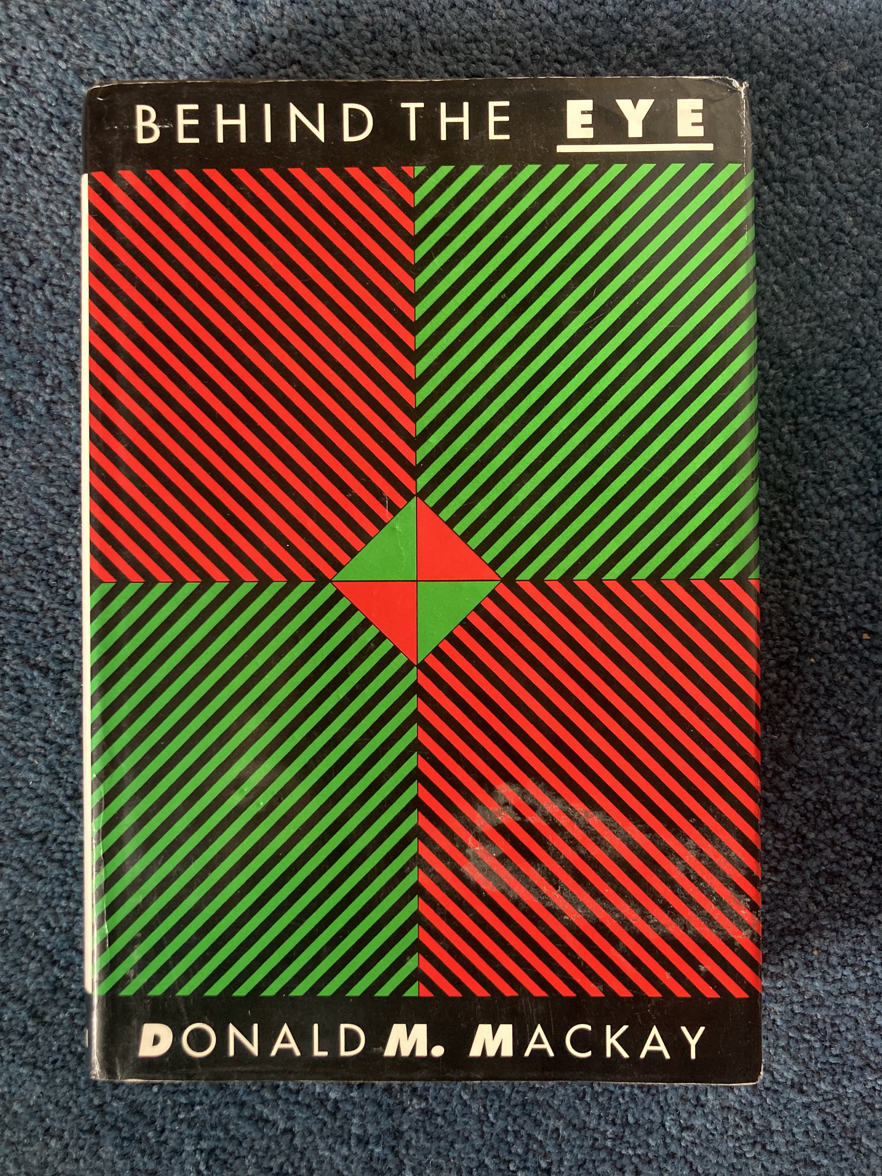
• Active sensing through rapid eye movements (saccades)
  • Not passive reception
  • Actively construct understanding
  • Hundreds of samples per second

Behind the Eye

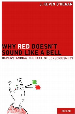
Visualization and Human Perception

• Visualization is powerful for communication
• But can be vulnerable to manipulation
  • Similar to social media algorithms
  • Misleading visualizations can deceive
  • Can hijack natural visual processing

Part 1: Discrete Latent Variables

Clustering

Clustering

• Common approach for grouping data points
• Assigns data points to discrete groups
• Examples include:
  • Animal classification
  • Political affiliation grouping

Clustering vs Vector Quantisation

• Clustering expects gaps between groups in data density
• Vector quantization may not require density gaps
• For practical purposes, both involve:
  • Allocating points to groups
  • Determining optimal number of groups

\(k\)-means Clustering

• Simple iterative clustering algorithm
• Key steps:
  1. Initialize with random centers
  2. Assign points to nearest center
  3. Update centers as cluster means
  4. Repeat until stable

Objective Function

• Minimizes sum of squared distances: \[ E=\sum_{j=1}^K \sum_{i\ \text{allocated to}\ j} \left(\mathbf{ y}_{i, :} - \boldsymbol{ \mu}_{j, :}\right)^\top\left(\mathbf{ y}_{i, :} - \boldsymbol{ \mu}_{j, :}\right) \]

• Solution not guaranteed to be global or unique

• Represents a non-convex optimization problem

• Task: associate data points with different labels.

• Labels are not provided by humans.

• Process is intuitive for humans - we do it naturally.

Platonic Ideals

• Greek philosopher Plato considered the concept of ideals
• The Platonic ideal bird is the most bird-like bird
• In clustering, we find these ideals as cluster centers
• Data points are allocated to their nearest center

Mathematical Formulation

• Represent objects as data vectors \(\mathbf{ x}_i\)
• Represent cluster centers as vectors \(\boldsymbol{ \mu}_j\)
• Define similarity/distance between objects and centers
• Distance function: \(d_{ij} = f(\mathbf{ x}_i, \boldsymbol{ \mu}_j)\)

Squared Distance

• Common choice: squared distance \[ d_{ij} = (\mathbf{ x}_i - \boldsymbol{ \mu}_j)^2 \]
• Goal: find centers close to many data points

Objective Function

• Given similarity measure, need number of cluster centers, \(K\).
• Find their location by allocating each center to a sub-set of the points and minimizing the sum of the squared errors, \[ E(\mathbf{M}) = \sum_{i \in \mathbf{i}_j} (\mathbf{ x}_i - \boldsymbol{ \mu}_j)^2 \] here \(\mathbf{i}_j\) is all indices of data points allocated to the \(j\)th center.

\(k\)-Means Clustering

• \(k\)-means clustering is simple and quick to implement.
• Very initialisation sensitive.

Initialisation

• Initialisation is the process of selecting a starting set of parameters.
• Optimisation result can depend on the starting point.
• For \(k\)-means clustering you need to choose an initial set of centers.
• Optimisation surface has many local optima, algorithm gets stuck in ones near initialisation.

\(k\)-Means Clustering

❮ ❯

Clustering with the \(k\)-means clustering algorithm.

\(k\)-Means Clustering

\(k\)-means clustering by Alex Ihler

Hierarchical Clustering

• Form taxonomies of the cluster centers
• Like humans apply to animals, to form phylogenies
• Builds a tree structure showing relationships between data points
• Two main approaches:
  • Agglomerative (bottom-up): Start with individual points and merge
  • Divisive (top-down): Start with one cluster and split

Oil Flow Data

}

Phylogenetic Trees

• Hierarchical clustering of genetic sequence data
• Creates evolutionary trees showing species relationships
• Estimates common ancestors and mutation timelines
• Critical for tracking viral evolution and outbreaks

Product Clustering

• Hierarchical clustering for e-commerce products
• Creates product taxonomy trees
• Splits into nested categories (e.g. Electronics → Phones → Smartphones)

Hierarchical Clustering Challenge

• Many products belong in multiple clusters (e.g. running shoes are both ‘sporting goods’ and ‘clothing’)
• Tree structures are too rigid for natural categorization
• Human concept learning is more flexible:
  • Forms overlapping categories
  • Learns abstract rules
  • Builds causal theories

Other Clustering Approaches

• Spectral clustering: Graph-based non-convex clustering
• Dirichlet process: Infinite, non-parametric clustering

Part 2: Continuous Latent Variables

High Dimensional Data

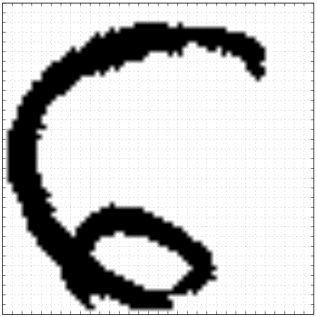
• USPS Data Set Handwritten Digit
• 3648 dimensions (64 rows, 57 columns)
• Space contains much more than just this digit.

USPS Samples

❮ ❯

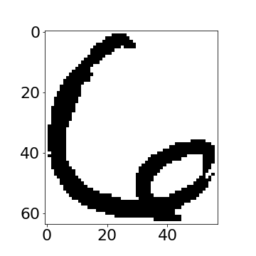
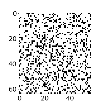
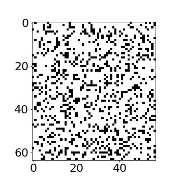
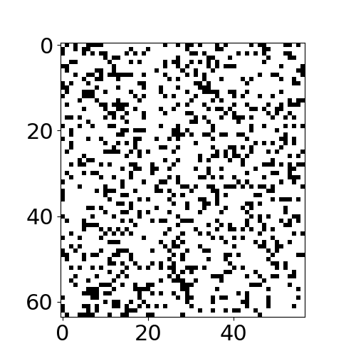
• Even if we sample every nanonsecond from now until end of universe you won’t see original six!

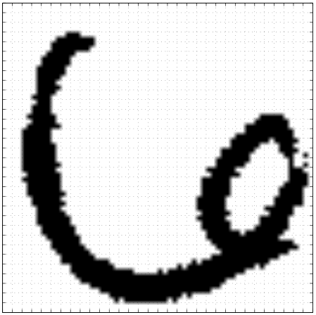
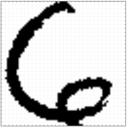
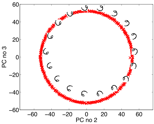
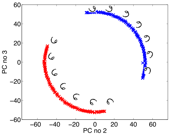
Simple Model of Digit

• Rotate a prototype

❮ ❯

Low Dimensional Manifolds

• Pure rotation is too simple
  • In practice data may undergo several distortions.
• For high dimensional data with structure:
  • We expect fewer distortions than dimensions;
  • Therefore we expect the data to live on a lower dimensional manifold.
  • Conclusion: Deal with high dimensional data by looking for a lower dimensional non-linear embedding.

High Dimensional Data Effects

• High dimensional spaces behave very differently from our 3D intuitions
• Two key effects:
  • Data moves to a “shell” at one standard deviation from mean
  • Distances between points become constant
• Let’s see this experimentally

Pairwise Distances in High-D Gaussian Data

Pairwise Distances in High-D Gaussian Data

• Plot shows pairwise distances in high-D Gaussian data
• Red line: theoretical gamma distribution
• Notice tight concentration of distances

Structured High Dimensional Data

• What about data with underlying structure?
• Let’s create data that lies on a 2D manifold
• Embed it in 1000D space

Pairwise Distances in Structured High-D Data

Pairwise Distances in Structured High-D Data

• Distance distribution differs from pure high-D case
• Matches 2D theoretical curve better than 1000D
• Real data often has low intrinsic dimensionality
• This is why PCA and other dimension reduction works!

High Dimensional Effects in Real Data

Oil Flow Data

Implications for Dimensionality Reduction

Latent Variables and Dimensionality Reduction

• Real data often has lower intrinsic dimensionality than measurements
• Examples:
  • Motion capture: Many coordinates but few degrees of freedom
  • Genetic data: Thousands of genes controlled by few regulators
  • Images: Millions of pixels but simpler underlying structure

Latent Variable Example

Latent Variable Example

• Example shows 2D data described by 1D latent variable
• Left: Data in original 2D space
• Right: Same data represented by single latent variable \(z\)
• Goal: Find these simpler underlying representations

Latent Variables

Your Personality

Factor Analysis Model

\[ \mathbf{ y}= \mathbf{f}(\mathbf{ z}) + \boldsymbol{ \epsilon}, \]

\[ \mathbf{f}(\mathbf{ z}) = \mathbf{W}\mathbf{ z} \]

Closely Related to Linear Regression

\[ \mathbf{f}(\mathbf{ z}) = \begin{bmatrix} f_1(\mathbf{ z}) \\ f_2(\mathbf{ z}) \\ \vdots \\ f_p(\mathbf{ z})\end{bmatrix} \]

\[ f_j(\mathbf{ z}) = \mathbf{ w}_{j, :}^\top \mathbf{ z}, \]

\[ \epsilon_j \sim \mathcal{N}\left(0,\sigma^2_j\right). \]

Data Representation

\[ \mathbf{Y} = \begin{bmatrix} \mathbf{ y}_{1, :}^\top \\ \mathbf{ y}_{2, :}^\top \\ \vdots \\ \mathbf{ y}_{n, :}^\top\end{bmatrix}, \]

\[ \mathbf{F} = \mathbf{Z}\mathbf{W}^\top, \]

Latent Variables vs Linear Regression

\[ x_{i,j} \sim \mathcal{N}\left(0,1\right), \] and we can write the density governing the latent variable associated with a single point as, \[ \mathbf{ z}_{i, :} \sim \mathcal{N}\left(\mathbf{0},\mathbf{I}\right). \]

\[ \mathbf{f}_{i, :} = \mathbf{f}(\mathbf{ z}_{i, :}) = \mathbf{W}\mathbf{ z}_{i, :} \]

\[ \mathbf{f}_{i, :} \sim \mathcal{N}\left(\mathbf{0},\mathbf{W}\mathbf{W}^\top\right) \]

Data Distribution

\[ \mathbf{ y}_{i, :} = \sim \mathcal{N}\left(\mathbf{0},\mathbf{W}\mathbf{W}^\top + \boldsymbol{\Sigma}\right) \]

\[ \boldsymbol{\Sigma} = \begin{bmatrix}\sigma^2_{1} & 0 & 0 & 0\\ 0 & \sigma^2_{2} & 0 & 0\\ 0 & 0 & \ddots & 0\\ 0 & 0 & 0 & \sigma^2_p\end{bmatrix}. \]

Mean Vector

\[ \mathbf{ y}_{i, :} = \mathbf{W}\mathbf{ z}_{i, :} + \boldsymbol{ \mu}+ \boldsymbol{ \epsilon}_{i, :} \]

\[ \boldsymbol{ \mu}= \frac{1}{n} \sum_{i=1}^n \mathbf{ y}_{i, :}, \] \(\mathbf{C}= \mathbf{W}\mathbf{W}^\top + \boldsymbol{\Sigma}\)

Principal Component Analysis

Hotelling (1933) took \(\sigma^2_i \rightarrow 0\) so \[ \mathbf{ y}_{i, :} \sim \lim_{\sigma^2 \rightarrow 0} \mathcal{N}\left(\mathbf{0},\mathbf{W}\mathbf{W}^\top + \sigma^2 \mathbf{I}\right). \]

Degenerate Covariance

\[ p(\mathbf{ y}_{i, :}|\mathbf{W}) = \lim_{\sigma^2 \rightarrow 0} \frac{1}{(2\pi)^\frac{p}{2} |\mathbf{W}\mathbf{W}^\top + \sigma^2 \mathbf{I}|^{\frac{1}{2}}} \exp\left(-\frac{1}{2}\mathbf{ y}_{i, :}\left[\mathbf{W}\mathbf{W}^\top+ \sigma^2 \mathbf{I}\right]^{-1}\mathbf{ y}_{i, :}\right), \]

Computation of the Marginal Likelihood

\[ \mathbf{ y}_{i,:}=\mathbf{W}\mathbf{ z}_{i,:}+\boldsymbol{ \epsilon}_{i,:},\quad \mathbf{ z}_{i,:} \sim \mathcal{N}\left(\mathbf{0},\mathbf{I}\right), \quad \boldsymbol{ \epsilon}_{i,:} \sim \mathcal{N}\left(\mathbf{0},\sigma^{2}\mathbf{I}\right) \]

\[ \mathbf{W}\mathbf{ z}_{i,:} \sim \mathcal{N}\left(\mathbf{0},\mathbf{W}\mathbf{W}^\top\right) \]

\[ \mathbf{W}\mathbf{ z}_{i, :} + \boldsymbol{ \epsilon}_{i, :} \sim \mathcal{N}\left(\mathbf{0},\mathbf{W}\mathbf{W}^\top + \sigma^2 \mathbf{I}\right) \]

Linear Latent Variable Model II

Probabilistic PCA Max. Likelihood Soln (Tipping and Bishop (1999))

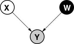
\[p\left(\mathbf{Y}|\mathbf{W}\right)=\prod_{i=1}^{n}\mathcal{N}\left(\mathbf{ y}_{i, :}|\mathbf{0},\mathbf{W}\mathbf{W}^{\top}+\sigma^{2}\mathbf{I}\right)\]

Linear Latent Variable Model II

Probabilistic PCA Max. Likelihood Soln (Tipping and Bishop (1999)) \[ p\left(\mathbf{Y}|\mathbf{W}\right)=\prod_{i=1}^{n}\mathcal{N}\left(\mathbf{ y}_{i,:}|\mathbf{0},\mathbf{C}\right),\quad \mathbf{C}=\mathbf{W}\mathbf{W}^{\top}+\sigma^{2}\mathbf{I} \] \[ \log p\left(\mathbf{Y}|\mathbf{W}\right)=-\frac{n}{2}\log\left|\mathbf{C}\right|-\frac{1}{2}\text{tr}\left(\mathbf{C}^{-1}\mathbf{Y}^{\top}\mathbf{Y}\right)+\text{const.} \] If \(\mathbf{U}_{q}\) are first \(q\) principal eigenvectors of \(n^{-1}\mathbf{Y}^{\top}\mathbf{Y}\) and the corresponding eigenvalues are \(\boldsymbol{\Lambda}_{q}\), \[ \mathbf{W}=\mathbf{U}_{q}\mathbf{L}\mathbf{R}^{\top},\quad\mathbf{L}=\left(\boldsymbol{\Lambda}_{q}-\sigma^{2}\mathbf{I}\right)^{\frac{1}{2}} \] where \(\mathbf{R}\) is an arbitrary rotation matrix.