Abstract

In this review and refresher notebook we remind ourselves about linear models and use the opportunity to provide some review of linear algebra. Most of the code you need is provided in the notebook, there are a few exercises to help develop your understanding.

Introduction

Welcome to the review and refresh practical. This work is for you to remind yourself about the ways of using the notebook. You will have a chance to ask us questions about the content on 9th of November. Within the material you will find exercises. If you are confident with probability you can likely ignore the reading and exercises which are listed from Rogers and Girolami (2011) and Bishop (2006). There should be no need to purchase these books for this course. The suggestions of sections are there just as a reminder.

We suggest you run these labs in Google colab, there’s a link to doing that on the main lab page at the top. We also suggest that the first thing you do is click View->Expand sections to make all parts of the lab visibile.

We suggest you complete at least Exercises 2-5.

Setup

notutils

This small package is a helper package for various notebook utilities used below.

The software can be installed using

%pip install notutils

from the command prompt where you can access your python installation.

The code is also available on GitHub: https://github.com/lawrennd/notutils

Once notutils is installed, it can be imported in the usual manner.

import notutils

pods

In Sheffield we created a suite of software tools for ‘Open Data Science’. Open data science is an approach to sharing code, models and data that should make it easier for companies, health professionals and scientists to gain access to data science techniques.

You can also check this blog post on Open Data Science.

The software can be installed using

%pip install pods

from the command prompt where you can access your python installation.

The code is also available on GitHub: https://github.com/lawrennd/ods

Once pods is installed, it can be imported in the usual manner.

import pods

mlai

The mlai software is a suite of helper functions for teaching and demonstrating machine learning algorithms. It was first used in the Machine Learning and Adaptive Intelligence course in Sheffield in 2013.

The software can be installed using

%pip install mlai

from the command prompt where you can access your python installation.

The code is also available on GitHub: https://github.com/lawrennd/mlai

Once mlai is installed, it can be imported in the usual manner.

import mlai

Review

• Last time: Looked at objective functions for movie recommendation.
• Minimized sum of squares objective by steepest descent and stochastic gradients.
• This time: explore least squares for regression.

Regression Examples

Regression involves predicting a real value, \(y_i\), given an input vector, \(\mathbf{ x}_i\). For example, the Tecator data involves predicting the quality of meat given spectral measurements. Or in radiocarbon dating, the C14 calibration curve maps from radiocarbon age to age measured through a back-trace of tree rings. Regression has also been used to predict the quality of board game moves given expert rated training data.

Olympic 100m Data

Gold medal times for Olympic 100 m runners since 1896. One of a number of Olypmic data sets collected by Rogers and Girolami (2011).

Figure: Start of the 2012 London 100m race. Image from Wikimedia Commons http://bit.ly/191adDC

The first thing we will do is load a standard data set for regression modelling. The data consists of the pace of Olympic Gold Medal 100m winners for the Olympics from 1896 to present. First we load in the data and plot.

import numpy as np
import pods

data = pods.datasets.olympic_100m_men()
x = data['X']
y = data['Y']

offset = y.mean()
scale = np.sqrt(y.var())

Figure: Olympic 100m wining times since 1896.

Olympic Marathon Data

Gold medal times for Olympic Marathon since 1896. Marathons before 1924 didn’t have a standardized distance. Present results using pace per km. In 1904 Marathon was badly organized leading to very slow times.

Image from Wikimedia Commons http://bit.ly/16kMKHQ

The first thing we will do is load a standard data set for regression modelling. The data consists of the pace of Olympic Gold Medal Marathon winners for the Olympics from 1896 to present. Let’s load in the data and plot.

import numpy as np
import pods

data = pods.datasets.olympic_marathon_men()
x = data['X']
y = data['Y']

offset = y.mean()
scale = np.sqrt(y.var())
yhat = (y - offset)/scale

Figure: Olympic marathon pace times since 1896.

Things to notice about the data include the outlier in 1904, in that year the Olympics was in St Louis, USA. Organizational problems and challenges with dust kicked up by the cars following the race meant that participants got lost, and only very few participants completed. More recent years see more consistently quick marathons.

What is Machine Learning?

What is machine learning? At its most basic level machine learning is a combination of

\[\text{data} + \text{model} \stackrel{\text{compute}}{\rightarrow} \text{prediction}\]

where data is our observations. They can be actively or passively acquired (meta-data). The model contains our assumptions, based on previous experience. That experience can be other data, it can come from transfer learning, or it can merely be our beliefs about the regularities of the universe. In humans our models include our inductive biases. The prediction is an action to be taken or a categorization or a quality score. The reason that machine learning has become a mainstay of artificial intelligence is the importance of predictions in artificial intelligence. The data and the model are combined through computation.

In practice we normally perform machine learning using two functions. To combine data with a model we typically make use of:

a prediction function it is used to make the predictions. It includes our beliefs about the regularities of the universe, our assumptions about how the world works, e.g., smoothness, spatial similarities, temporal similarities.

an objective function it defines the ‘cost’ of misprediction. Typically, it includes knowledge about the world’s generating processes (probabilistic objectives) or the costs we pay for mispredictions (empirical risk minimization).

The combination of data and model through the prediction function and the objective function leads to a learning algorithm. The class of prediction functions and objective functions we can make use of is restricted by the algorithms they lead to. If the prediction function or the objective function are too complex, then it can be difficult to find an appropriate learning algorithm. Much of the academic field of machine learning is the quest for new learning algorithms that allow us to bring different types of models and data together.

A useful reference for state of the art in machine learning is the UK Royal Society Report, Machine Learning: Power and Promise of Computers that Learn by Example.

You can also check my post blog post on What is Machine Learning?.

Sum of Squares Error

Last week we considered a cost function for minimization of the error. We considered items (films) and users and assumed that each movie rating, \(y_{i,j}\) could be summarised by an inner product between a vector associated with the item, \(\mathbf{v}_j\) and one associated with the user \(\mathbf{u}_i\). We justified the inner product as a measure of similarity in the space of ‘movie subjects’, where both the users and the items lived, giving the analogy of a library.

To make predictions we encouraged the similarity to be high if the movie rating was high using the quadratic error function, \[ E_{i,j}(\mathbf{u}_i, \mathbf{v}_j) = \left(\mathbf{u}_i^\top \mathbf{v}_j - y_{i,j}\right)^2, \] which we then summed across all the observations to form the total error \[ E(\mathbf{U}, \mathbf{V}) = \sum_{i,j}s_{i,j}\left(\mathbf{u}_i^\top \mathbf{v}_j - y_{i,j}\right)^2, \] where \(s_{i,j}\) is an indicator variable which is set to 1 if the rating of movie \(j\) by user \(i\) is provided in our data set. This is known as a sum of squares error.

This week we will reinterpret the error as a probabilistic model. We will consider the difference between our data and our model to have come from unconsidered factors which exhibit as a probability density. This leads to a more principled definition of least squares error that is originally due to Carl Friederich Gauss, but is mainly inspired by the thinking of Pierre-Simon Laplace.

Regression: Linear Releationship

For many their first encounter with what might be termed a machine learning method is fitting a straight line. A straight line is characterized by two parameters, the scale, \(m\), and the offset \(c\).

\[y_i = m x_i + c\]

For the olympic marathon example \(y_i\) is the winning pace and it is given as a function of the year which is represented by \(x_i\). There are two further parameters of the prediction function. For the olympics example we can interpret these parameters, the scale \(m\) is the rate of improvement of the olympic marathon pace on a yearly basis. And \(c\) is the winning pace as estimated at year 0.

Overdetermined System

The challenge with a linear model is that it has two unknowns, \(m\), and \(c\). Observing data allows us to write down a system of simultaneous linear equations. So, for example if we observe two data points, the first with the input value, \(x_1 = 1\) and the output value, \(y_1 =3\) and a second data point, \(x= 3\), \(y=1\), then we can write two simultaneous linear equations of the form.

point 1: \(x= 1\), \(y=3\) \[ 3 = m + c \] point 2: \(x= 3\), \(y=1\) \[ 1 = 3m + c \]

The solution to these two simultaneous equations can be represented graphically as

Figure: The solution of two linear equations represented as the fit of a straight line through two data

The challenge comes when a third data point is observed, and it doesn’t fit on the straight line.

point 3: \(x= 2\), \(y=2.5\) \[ 2.5 = 2m + c \]

Figure: A third observation of data is inconsistent with the solution dictated by the first two observations

Now there are three candidate lines, each consistent with our data.

Figure: Three solutions to the problem, each consistent with two points of the three observations

This is known as an overdetermined system because there are more data than we need to determine our parameters. The problem arises because the model is a simplification of the real world, and the data we observe is therefore inconsistent with our model.

Pierre-Simon Laplace

The solution was proposed by Pierre-Simon Laplace. His idea was to accept that the model was an incomplete representation of the real world, and the way it was incomplete is unknown. His idea was that such unknowns could be dealt with through probability.

Pierre-Simon Laplace

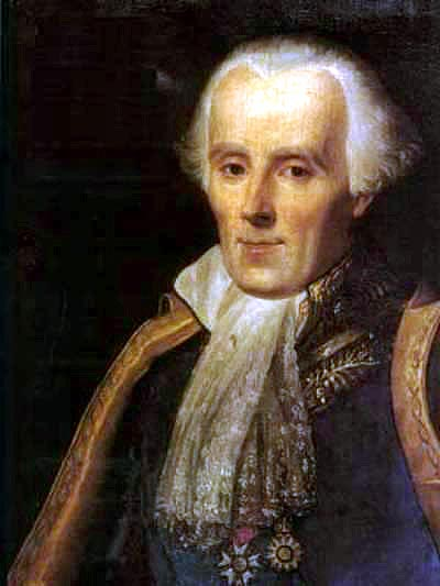
Figure: Pierre-Simon Laplace 1749-1827.

Famously, Laplace considered the idea of a deterministic Universe, one in which the model is known, or as the below translation refers to it, “an intelligence which could comprehend all the forces by which nature is animated”. He speculates on an “intelligence” that can submit this vast data to analysis and propsoses that such an entity would be able to predict the future.

Given for one instant an intelligence which could comprehend all the forces by which nature is animated and the respective situation of the beings who compose it—an intelligence sufficiently vast to submit these data to analysis—it would embrace in the same formulate the movements of the greatest bodies of the universe and those of the lightest atom; for it, nothing would be uncertain and the future, as the past, would be present in its eyes.

This notion is known as Laplace’s demon or Laplace’s superman.

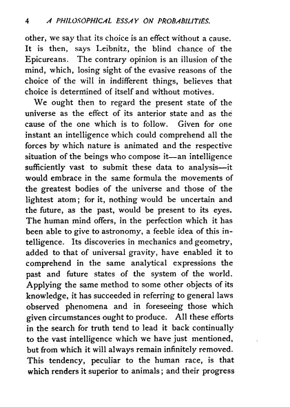
Figure: Laplace’s determinsim in English translation.

Laplace’s Gremlin

Unfortunately, most analyses of his ideas stop at that point, whereas his real point is that such a notion is unreachable. Not so much superman as strawman. Just three pages later in the “Philosophical Essay on Probabilities” (Laplace, 1814), Laplace goes on to observe:

The curve described by a simple molecule of air or vapor is regulated in a manner just as certain as the planetary orbits; the only difference between them is that which comes from our ignorance.

Probability is relative, in part to this ignorance, in part to our knowledge.

Figure: To Laplace, determinism is a strawman. Ignorance of mechanism and data leads to uncertainty which should be dealt with through probability.

In other words, we can never make use of the idealistic deterministic Universe due to our ignorance about the world, Laplace’s suggestion, and focus in this essay is that we turn to probability to deal with this uncertainty. This is also our inspiration for using probability in machine learning. This is the true message of Laplace’s essay, not determinism, but the gremlin of uncertainty that emerges from our ignorance.

The “forces by which nature is animated” is our model, the “situation of beings that compose it” is our data and the “intelligence sufficiently vast enough to submit these data to analysis” is our compute. The fly in the ointment is our ignorance about these aspects. And probability is the tool we use to incorporate this ignorance leading to uncertainty or doubt in our predictions.

Latent Variables

Laplace’s concept was that the reason that the data doesn’t match up to the model is because of unconsidered factors, and that these might be well represented through probability densities. He tackles the challenge of the unknown factors by adding a variable, \(\epsilon\), that represents the unknown. In modern parlance we would call this a latent variable. But in the context Laplace uses it, the variable is so common that it has other names such as a “slack” variable or the noise in the system.

point 1: \(x= 1\), \(y=3\) [ 3 = m + c + _1 ] point 2: \(x= 3\), \(y=1\) [ 1 = 3m + c + _2 ] point 3: \(x= 2\), \(y=2.5\) [ 2.5 = 2m + c + _3 ]

Laplace’s trick has converted the overdetermined system into an underdetermined system. He has now added three variables, \(\{\epsilon_i\}_{i=1}^3\), which represent the unknown corruptions of the real world. Laplace’s idea is that we should represent that unknown corruption with a probability distribution.

A Probabilistic Process

However, it was left to an admirer of Laplace to develop a practical probability density for that purpose. It was Carl Friedrich Gauss who suggested that the Gaussian density (which at the time was unnamed!) should be used to represent this error.

The result is a noisy function, a function which has a deterministic part, and a stochastic part. This type of function is sometimes known as a probabilistic or stochastic process, to distinguish it from a deterministic process.

The Gaussian Density

The Gaussian density is perhaps the most commonly used probability density. It is defined by a mean, \(\mu\), and a variance, \(\sigma^2\). The variance is taken to be the square of the standard deviation, \(\sigma\).

\[\begin{align} p(y| \mu, \sigma^2) & = \frac{1}{\sqrt{2\pi\sigma^2}}\exp\left(-\frac{(y- \mu)^2}{2\sigma^2}\right)\\& \buildrel\triangle\over = \mathcal{N}\left(y|\mu,\sigma^2\right) \end{align}\]

Figure: The Gaussian PDF with \({\mu}=1.7\) and variance \({\sigma}^2=0.0225\). Mean shown as red line. It could represent the heights of a population of students.

Two Important Gaussian Properties

The Gaussian density has many important properties, but for the moment we’ll review two of them.

Sum of Gaussians

If we assume that a variable, \(y_i\), is sampled from a Gaussian density,

\[y_i \sim \mathcal{N}\left(\mu_i,\sigma_i^2\right)\]

Then we can show that the sum of a set of variables, each drawn independently from such a density is also distributed as Gaussian. The mean of the resulting density is the sum of the means, and the variance is the sum of the variances,

\[ \sum_{i=1}^{n} y_i \sim \mathcal{N}\left(\sum_{i=1}^n\mu_i,\sum_{i=1}^n\sigma_i^2\right) \]

Since we are very familiar with the Gaussian density and its properties, it is not immediately apparent how unusual this is. Most random variables, when you add them together, change the family of density they are drawn from. For example, the Gaussian is exceptional in this regard. Indeed, other random variables, if they are independently drawn and summed together tend to a Gaussian density. That is the central limit theorem which is a major justification for the use of a Gaussian density.

Scaling a Gaussian

Less unusual is the scaling property of a Gaussian density. If a variable, \(y\), is sampled from a Gaussian density,

\[y\sim \mathcal{N}\left(\mu,\sigma^2\right)\] and we choose to scale that variable by a deterministic value, \(w\), then the scaled variable is distributed as

\[wy\sim \mathcal{N}\left(w\mu,w^2 \sigma^2\right).\] Unlike the summing properties, where adding two or more random variables independently sampled from a family of densitites typically brings the summed variable outside that family, scaling many densities leaves the distribution of that variable in the same family of densities. Indeed, many densities include a scale parameter (e.g. the Gamma density) which is purely for this purpose. In the Gaussian the standard deviation, \(\sigma\), is the scale parameter. To see why this makes sense, let’s consider, \[z \sim \mathcal{N}\left(0,1\right),\] then if we scale by \(\sigma\) so we have, \(y=\sigma z\), we can write, \[y=\sigma z \sim \mathcal{N}\left(0,\sigma^2\right)\]

Laplace’s Idea

Laplace had the idea to augment the observations by noise, that is equivalent to considering a probability density whose mean is given by the prediction function \[p\left(y_i|x_i\right)=\frac{1}{\sqrt{2\pi\sigma^2}}\exp\left(-\frac{\left(y_i-f\left(x_i\right)\right)^{2}}{2\sigma^2}\right).\]

This is known as stochastic process. It is a function that is corrupted by noise. Laplace didn’t suggest the Gaussian density for that purpose, that was an innovation from Carl Friederich Gauss, which is what gives the Gaussian density its name.

Height as a Function of Weight

In the standard Gaussian, parameterized by mean and variance, make the mean a linear function of an input.

This leads to a regression model. \[ \begin{align*} y_i=&f\left(x_i\right)+\epsilon_i,\\ \epsilon_i \sim & \mathcal{N}\left(0,\sigma^2\right). \end{align*} \]

Assume \(y_i\) is height and \(x_i\) is weight.

Sum of Squares Error

Legendre

Minimizing the sum of squares error was first proposed by Legendre in 1805 (Legendre, 1805). His book, which was on the orbit of comets, is available on google books, we can take a look at the relevant page by calling the code below.

Figure: Legendre’s book was on the determination of orbits of comets. This page describes the formulation of least squares

Of course, the main text is in French, but the key part we are interested in can be roughly translated as

In most matters where we take measures data through observation, the most accurate results they can offer, it is almost always leads to a system of equations of the form \[E = a + bx + cy + fz + etc .\] where \(a\), \(b\), \(c\), \(f\) etc are the known coefficients and \(x\), \(y\), \(z\) etc are unknown and must be determined by the condition that the value of E is reduced, for each equation, to an amount or zero or very small.

He continues

Of all the principles that we can offer for this item, I think it is not broader, more accurate, nor easier than the one we have used in previous research application, and that is to make the minimum sum of the squares of the errors. By this means, it is between the errors a kind of balance that prevents extreme to prevail, is very specific to make known the state of the closest to the truth system. The sum of the squares of the errors \(E^2 + \left.E^\prime\right.^2 + \left.E^{\prime\prime}\right.^2 + etc\) being \[\begin{align*} &(a + bx + cy + fz + etc)^2 \\ + &(a^\prime + b^\prime x + c^\prime y + f^\prime z + etc ) ^2\\ + &(a^{\prime\prime} + b^{\prime\prime}x + c^{\prime\prime}y + f^{\prime\prime}z + etc )^2 \\ + & etc \end{align*}\] if we wanted a minimum, by varying x alone, we will have the equation …

This is the earliest know printed version of the problem of least squares. The notation, however, is a little awkward for mordern eyes. In particular Legendre doesn’t make use of the sum sign, \[ \sum_{i=1}^3 z_i = z_1 + z_2 + z_3 \] nor does he make use of the inner product.

In our notation, if we were to do linear regression, we would need to subsititue: \[\begin{align*} a &\leftarrow y_1-c, \\ a^\prime &\leftarrow y_2-c,\\ a^{\prime\prime} &\leftarrow y_3 -c,\\ \text{etc.} \end{align*}\] to introduce the data observations \(\{y_i\}_{i=1}^{n}\) alongside \(c\), the offset. We would then introduce the input locations \[\begin{align*} b & \leftarrow x_1,\\ b^\prime & \leftarrow x_2,\\ b^{\prime\prime} & \leftarrow x_3\\ \text{etc.} \end{align*}\] and finally the gradient of the function \[x \leftarrow -m.\] The remaining coefficients (\(c\) and \(f\)) would then be zero. That would give us \[\begin{align*} &(y_1 - (mx_1+c))^2 \\ + &(y_2 -(mx_2 + c))^2\\ + &(y_3 -(mx_3 + c))^2 \\ + & \text{etc.} \end{align*}\] which we would write in the modern notation for sums as \[ \sum_{i=1}^n(y_i-(mx_i + c))^2 \] which is recognised as the sum of squares error for a linear regression.

This shows the advantage of modern summation operator, \(\sum\), in keeping our mathematical notation compact. Whilst it may look more complicated the first time you see it, understanding the mathematical rules that go around it, allows us to go much further with the notation.

Inner products (or dot products) are similar. They allow us to write \[ \sum_{i=1}^q u_i v_i \] in a more compact notation, \(\mathbf{u}\cdot\mathbf{v}.\)

Here we are using bold face to represent vectors, and we assume that the individual elements of a vector \(\mathbf{z}\) are given as a series of scalars \[ \mathbf{z} = \begin{bmatrix} z_1\\ z_2\\ \vdots\\ z_n \end{bmatrix} \] which are each indexed by their position in the vector.

Running Example: Olympic Marathons

Note that x and y are not pandas data frames for this example, they are just arrays of dimensionality \(n\times 1\), where \(n\) is the number of data.

The aim of this lab is to have you coding linear regression in python. We will do it in two ways, once using iterative updates (coordinate ascent) and then using linear algebra. The linear algebra approach will not only work much better, it is also easy to extend to multiple input linear regression and non-linear regression using basis functions.

Maximum Likelihood: Iterative Solution

Now we will take the maximum likelihood approach we derived in the lecture to fit a line, \(y_i=mx_i + c\), to the data you’ve plotted. We are trying to minimize the error function: \[ E(m, c) = \sum_{i=1}^n(y_i-mx_i-c)^2 \] with respect to \(m\), \(c\) and \(\sigma^2\). We can start with an initial guess for \(m\),

m = -0.4
c = 80

Then we use the maximum likelihood update to find an estimate for the offset, \(c\).

Coordinate Descent

In the movie recommender system example, we minimised the objective function by steepest descent based gradient methods. Our updates required us to compute the gradient at the position we were located, then to update the gradient according to the direction of steepest descent. This time, we will take another approach. It is known as coordinate descent. In coordinate descent, we choose to move one parameter at a time. Ideally, we design an algorithm that at each step moves the parameter to its minimum value. At each step we choose to move the individual parameter to its minimum.

To find the minimum, we look for the point in the curve where the gradient is zero. This can be found by taking the gradient of \(E(m,c)\) with respect to the parameter.

Update for Offset

Let’s consider the parameter \(c\) first. The gradient goes nicely through the summation operator, and we obtain \[ \frac{\text{d}E(m,c)}{\text{d}c} = -\sum_{i=1}^n2(y_i-mx_i-c). \] Now we want the point that is a minimum. A minimum is an example of a stationary point, the stationary points are those points of the function where the gradient is zero. They are found by solving the equation for \(\frac{\text{d}E(m,c)}{\text{d}c} = 0\). Substituting in to our gradient, we can obtain the following equation, \[ 0 = -\sum_{i=1}^n2(y_i-mx_i-c) \] which can be reorganised as follows, \[ c^* = \frac{\sum_{i=1}^n(y_i-m^*x_i)}{n}. \] The fact that the stationary point is easily extracted in this manner implies that the solution is unique. There is only one stationary point for this system. Traditionally when trying to determine the type of stationary point we have encountered we now compute the second derivative, \[ \frac{\text{d}^2E(m,c)}{\text{d}c^2} = 2n. \] The second derivative is positive, which in turn implies that we have found a minimum of the function. This means that setting \(c\) in this way will take us to the lowest point along that axes.

# set c to the minimum
c = (y - m*x).mean()
print(c)

Update for Slope

Now we have the offset set to the minimum value, in coordinate descent, the next step is to optimise another parameter. Only one further parameter remains. That is the slope of the system.

Now we can turn our attention to the slope. We once again peform the same set of computations to find the minima. We end up with an update equation of the following form.

\[m^* = \frac{\sum_{i=1}^n(y_i - c)x_i}{\sum_{i=1}^nx_i^2}\]

Communication of mathematics in data science is an essential skill, in a moment, you will be asked to rederive the equation above. Before we do that, however, we will briefly review how to write mathematics in the notebook.

\(\LaTeX\) for Maths

These cells use Markdown format. You can include maths in your markdown using \(\LaTeX\) syntax, all you have to do is write your answer inside dollar signs, as follows:

To write a fraction, we write $\frac{a}{b}$, and it will display like this \(\frac{a}{b}\). To write a subscript we write $a_b$ which will appear as \(a_b\). To write a superscript (for example in a polynomial) we write $a^b$ which will appear as \(a^b\). There are lots of other macros as well, for example we can do greek letters such as $\alpha, \beta, \gamma$ rendering as \(\alpha, \beta, \gamma\). And we can do sum and intergral signs as $\sum \int \int$.

You can combine many of these operations together for composing expressions.

Exercise 1

Convert the following python code expressions into \(\LaTeX\)j, writing your answers below. In each case write your answer as a single equality (i.e. your maths should only contain one expression, not several lines of expressions). For the purposes of your \(\LaTeX\) please assume that x and w are \(n\) dimensional vectors.

(a) f = x.sum()

(b) m = x.mean()

(c) g = (x*w).sum()

Fixed Point Updates

\[ \begin{aligned} c^{*}=&\frac{\sum _{i=1}^{n}\left(y_i-m^{*}x_i\right)}{n},\\ m^{*}=&\frac{\sum _{i=1}^{n}x_i\left(y_i-c^{*}\right)}{\sum _{i=1}^{n}x_i^{2}},\\ \left.\sigma^2\right.^{*}=&\frac{\sum _{i=1}^{n}\left(y_i-m^{*}x_i-c^{*}\right)^{2}}{n} \end{aligned} \]

Gradient With Respect to the Slope

Now that you’ve had a little training in writing maths with \(\LaTeX\), we will be able to use it to answer questions. The next thing we are going to do is a little differentiation practice.

Exercise 2

Derive the the gradient of the objective function with respect to the slope, \(m\). Rearrange it to show that the update equation written above does find the stationary points of the objective function. By computing its derivative show that it’s a minimum.

m = ((y - c)*x).sum()/(x**2).sum()
print(m)

We can have a look at how good our fit is by computing the prediction across the input space. First create a vector of ‘test points’,

import numpy as np

x_test = np.linspace(1890, 2020, 130)[:, None]

Now use this vector to compute some test predictions,

f_test = m*x_test + c

Now plot those test predictions with a blue line on the same plot as the data,

import matplotlib.pyplot as plt

plt.plot(x_test, f_test, 'b-')
plt.plot(x, y, 'rx')

The fit isn’t very good, we need to iterate between these parameter updates in a loop to improve the fit, we have to do this several times,

for i in np.arange(10):
    m = ((y - c)*x).sum()/(x*x).sum()
    c = (y-m*x).sum()/y.shape[0]
print(m)
print(c)

And let’s try plotting the result again

f_test = m*x_test + c
plt.plot(x_test, f_test, 'b-')
plt.plot(x, y, 'rx')

Clearly we need more iterations than 10! In the next question you will add more iterations and report on the error as optimisation proceeds.

Exercise 3

There is a problem here, we seem to need many interations to get to a good solution. Let’s explore what’s going on. Write code which alternates between updates of c and m. Include the following features in your code.

1. Initialise with m=-0.4 and c=80.
2. Every 10 iterations compute the value of the objective function for the training data and print it to the screen (you’ll find hints on this in the lab from last week).
3. Cause the code to stop running when the error change over less than 10 iterations is smaller than \(1\times10^{-4}\). This is known as a stopping criterion.

Why do we need so many iterations to get to the solution?

Important Concepts Not Covered

• Other optimization methods:
  • Second order methods, conjugate gradient, quasi-Newton and Newton.
• Effective heuristics such as momentum.
• Local vs global solutions.

Objective Functions and Regression

import numpy as np
import matplotlib.pyplot as plt
import mlai

x = np.random.normal(size=(4, 1))

m_true = 1.4
c_true = -3.1

y = m_true*x+c_true

Figure: A simple linear regression.

Noise Corrupted Plot

noise = np.random.normal(scale=0.5, size=(4, 1)) # standard deviation of the noise is 0.5
y = m_true*x + c_true + noise
plt.plot(x, y, 'r.', markersize=10)
plt.xlim([-3, 3])
mlai.write_figure(filename='regression_noise.svg', directory='./ml', transparent=True)

Figure: A simple linear regression with noise.

Contour Plot of Error Function

• Visualise the error function surface, create vectors of values.

# create an array of linearly separated values around m_true
m_vals = np.linspace(m_true-3, m_true+3, 100) 
# create an array of linearly separated values ae
c_vals = np.linspace(c_true-3, c_true+3, 100)

• create a grid of values to evaluate the error function in 2D.

m_grid, c_grid = np.meshgrid(m_vals, c_vals)

• compute the error function at each combination of \(c\) and \(m\).

E_grid = np.zeros((100, 100))
for i in range(100):
    for j in range(100):
        E_grid[i, j] = ((y - m_grid[i, j]*x - c_grid[i, j])**2).sum()

Contour Plot of Error

Figure: Contours of the objective function for linear regression by minimizing least squares.

Steepest Descent

Algorithm

• We start with a guess for \(m\) and \(c\).

m_star = 0.0
c_star = -5.0

Offset Gradient

• Now we need to compute the gradient of the error function, firstly with respect to \(c\), \[ \frac{\text{d}E(m, c)}{\text{d} c} = -2\sum_{i=1}^n(y_i - mx_i - c) \]

• This is computed in python as follows

c_grad = -2*(y-m_star*x - c_star).sum()
print("Gradient with respect to c is ", c_grad)

Deriving the Gradient

To see how the gradient was derived, first note that the \(c\) appears in every term in the sum. So we are just differentiating \((y_i - mx_i - c)^2\) for each term in the sum. The gradient of this term with respect to \(c\) is simply the gradient of the outer quadratic, multiplied by the gradient with respect to \(c\) of the part inside the quadratic. The gradient of a quadratic is two times the argument of the quadratic, and the gradient of the inside linear term is just minus one. This is true for all terms in the sum, so we are left with the sum in the gradient.

Slope Gradient

The gradient with respect tom \(m\) is similar, but now the gradient of the quadratic’s argument is \(-x_i\) so the gradient with respect to \(m\) is

\[\frac{\text{d}E(m, c)}{\text{d} m} = -2\sum_{i=1}^nx_i(y_i - mx_i - c)\]

which can be implemented in python (numpy) as

m_grad = -2*(x*(y-m_star*x - c_star)).sum()
print("Gradient with respect to m is ", m_grad)

Update Equations

• Now we have gradients with respect to \(m\) and \(c\).
• Can update our inital guesses for \(m\) and \(c\) using the gradient.
• We don’t want to just subtract the gradient from \(m\) and \(c\),
• We need to take a small step in the gradient direction.
• Otherwise we might overshoot the minimum.
• We want to follow the gradient to get to the minimum, the gradient changes all the time.

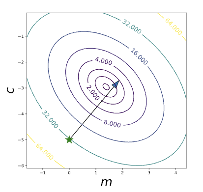
Move in Direction of Gradient

Figure: Single update descending the contours of the error surface for regression.

Update Equations

• The step size has already been introduced, it’s again known as the learning rate and is denoted by \(\eta\). \[ c_\text{new}\leftarrow c_{\text{old}} - \eta\frac{\text{d}E(m, c)}{\text{d}c} \]

• gives us an update for our estimate of \(c\) (which in the code we’ve been calling c_star to represent a common way of writing a parameter estimate, \(c^*\)) and \[ m_\text{new} \leftarrow m_{\text{old}} - \eta\frac{\text{d}E(m, c)}{\text{d}m} \]

• Giving us an update for \(m\).

Update Code

• These updates can be coded as

print("Original m was", m_star, "and original c was", c_star)
learn_rate = 0.01
c_star = c_star - learn_rate*c_grad
m_star = m_star - learn_rate*m_grad
print("New m is", m_star, "and new c is", c_star)

Iterating Updates

• Fit model by descending gradient.

Gradient Descent Algorithm

num_plots = plot.regression_contour_fit(x, y, diagrams='./ml')

Figure: Batch gradient descent for linear regression

Stochastic Gradient Descent

• If \(n\) is small, gradient descent is fine.
• But sometimes (e.g. on the internet \(n\) could be a billion.
• Stochastic gradient descent is more similar to perceptron.
• Look at gradient of one data point at a time rather than summing across all data points)
• This gives a stochastic estimate of gradient.

Stochastic Gradient Descent

• The real gradient with respect to \(m\) is given by

  \[\frac{\text{d}E(m, c)}{\text{d} m} = -2\sum_{i=1}^nx_i(y_i - mx_i - c)\]

  but it has \(n\) terms in the sum. Substituting in the gradient we can see that the full update is of the form

  \[m_\text{new} \leftarrow m_\text{old} + 2\eta\left[x_1 (y_1 - m_\text{old}x_1 - c_\text{old}) + (x_2 (y_2 - m_\text{old}x_2 - c_\text{old}) + \dots + (x_n (y_n - m_\text{old}x_n - c_\text{old})\right]\]

  This could be split up into lots of individual updates \[m_1 \leftarrow m_\text{old} + 2\eta\left[x_1 (y_1 - m_\text{old}x_1 - c_\text{old})\right]\] \[m_2 \leftarrow m_1 + 2\eta\left[x_2 (y_2 - m_\text{old}x_2 - c_\text{old})\right]\] \[m_3 \leftarrow m_2 + 2\eta \left[\dots\right]\] \[m_n \leftarrow m_{n-1} + 2\eta\left[x_n (y_n - m_\text{old}x_n - c_\text{old})\right]\]

which would lead to the same final update.

Updating \(c\) and \(m\)

• In the sum we don’t \(m\) and \(c\) we use for computing the gradient term at each update.
• In stochastic gradient descent we do change them.
• This means it’s not quite the same as steepest desceint.
• But we can present each data point in a random order, like we did for the perceptron.
• This makes the algorithm suitable for large scale web use (recently this domain is know as ‘Big Data’) and algorithms like this are widely used by Google, Microsoft, Amazon, Twitter and Facebook.

Stochastic Gradient Descent

• Or more accurate, since the data is normally presented in a random order we just can write \[ m_\text{new} = m_\text{old} + 2\eta\left[x_i (y_i - m_\text{old}x_i - c_\text{old})\right] \]

# choose a random point for the update 
i = np.random.randint(x.shape[0]-1)
# update m
m_star = m_star + 2*learn_rate*(x[i]*(y[i]-m_star*x[i] - c_star))
# update c
c_star = c_star + 2*learn_rate*(y[i]-m_star*x[i] - c_star)

SGD for Linear Regression

Putting it all together in an algorithm, we can do stochastic gradient descent for our regression data.

Figure: Stochastic gradient descent for linear regression.

Reflection on Linear Regression and Supervised Learning

Think about:

1. What effect does the learning rate have in the optimization? What’s the effect of making it too small, what’s the effect of making it too big? Do you get the same result for both stochastic and steepest gradient descent?

2. The stochastic gradient descent doesn’t help very much for such a small data set. It’s real advantage comes when there are many, you’ll see this in the lab.

Log Likelihood for Multivariate Regression

Quadratic Loss

Now we’ve identified the empirical risk with the loss, we’ll use \(E(\mathbf{ w})\) to represent our objective function. \[ E(\mathbf{ w}) = \sum_{i=1}^n\left(y_i - f(\mathbf{ x}_i, \mathbf{ w})\right)^2 \] gives us our objective.

In the case of the linear prediction function, we can substitute \(f(\mathbf{ x}_i, \mathbf{ w}) = \mathbf{ w}^\top \mathbf{ x}_i\). \[ E(\mathbf{ w}) = \sum_{i=1}^n\left(y_i - \mathbf{ w}^\top \mathbf{ x}_i\right)^2 \] To compute the gradient of the objective, we first expand the brackets.

Bracket Expansion

\[ \begin{align*} E(\mathbf{ w},\sigma^2) = & \frac{n}{2}\log \sigma^2 + \frac{1}{2\sigma^2}\sum _{i=1}^{n}y_i^{2}-\frac{1}{\sigma^2}\sum _{i=1}^{n}y_i\mathbf{ w}^{\top}\mathbf{ x}_i\\&+\frac{1}{2\sigma^2}\sum _{i=1}^{n}\mathbf{ w}^{\top}\mathbf{ x}_i\mathbf{ x}_i^{\top}\mathbf{ w} +\text{const}.\\ = & \frac{n}{2}\log \sigma^2 + \frac{1}{2\sigma^2}\sum _{i=1}^{n}y_i^{2}-\frac{1}{\sigma^2} \mathbf{ w}^\top\sum_{i=1}^{n}\mathbf{ x}_iy_i\\&+\frac{1}{2\sigma^2} \mathbf{ w}^{\top}\left[\sum _{i=1}^{n}\mathbf{ x}_i\mathbf{ x}_i^{\top}\right]\mathbf{ w}+\text{const}. \end{align*} \]

Solution with Linear Algebra

In this section we’re going compute the minimum of the quadratic loss with respect to the parameters. When we do this, we’ll also review linear algebra. We will represent all our errors and functions in the form of matrices and vectors.

Linear algebra is just a shorthand for performing lots of multiplications and additions simultaneously. What does it have to do with our system then? Well, the first thing to note is that the classic linear function we fit for a one-dimensional regression has the form: \[ f(x) = mx + c \] the classical form for a straight line. From a linear algebraic perspective, we are looking for multiplications and additions. We are also looking to separate our parameters from our data. The data is the givens. In French the word is données literally translated means givens that’s great, because we don’t need to change the data, what we need to change are the parameters (or variables) of the model. In this function the data comes in through \(x\), and the parameters are \(m\) and \(c\).

What we’d like to create is a vector of parameters and a vector of data. Then we could represent the system with vectors that represent the data, and vectors that represent the parameters.

We look to turn the multiplications and additions into a linear algebraic form, we have one multiplication (\(m\times c\)) and one addition (\(mx + c\)). But we can turn this into an inner product by writing it in the following way, \[ f(x) = m \times x + c \times 1, \] in other words, we’ve extracted the unit value from the offset, \(c\). We can think of this unit value like an extra item of data, because it is always given to us, and it is always set to 1 (unlike regular data, which is likely to vary!). We can therefore write each input data location, \(\mathbf{ x}\), as a vector \[ \mathbf{ x}= \begin{bmatrix} 1\\ x\end{bmatrix}. \]

Now we choose to also turn our parameters into a vector. The parameter vector will be defined to contain \[ \mathbf{ w}= \begin{bmatrix} c \\ m\end{bmatrix} \] because if we now take the inner product between these two vectors we recover \[ \mathbf{ x}\cdot\mathbf{ w}= 1 \times c + x \times m = mx + c \] In numpy we can define this vector as follows

import numpy as np

# define the vector w
w = np.zeros(shape=(2, 1))
w[0] = m
w[1] = c

This gives us the equivalence between original operation and an operation in vector space. Whilst the notation here isn’t a lot shorter, the beauty is that we will be able to add as many features as we like and keep the same representation. In general, we are now moving to a system where each of our predictions is given by an inner product. When we want to represent a linear product in linear algebra, we tend to do it with the transpose operation, so since we have \(\mathbf{a}\cdot\mathbf{b} = \mathbf{a}^\top\mathbf{b}\) we can write \[ f(\mathbf{ x}_i) = \mathbf{ x}_i^\top\mathbf{ w}. \] Where we’ve assumed that each data point, \(\mathbf{ x}_i\), is now written by appending a 1 onto the original vector \[ \mathbf{ x}_i = \begin{bmatrix} 1 \\ x_i \end{bmatrix} \]

Design Matrix

We can do this for the entire data set to form a design matrix \(\mathbf{X}\), \[ \mathbf{X} = \begin{bmatrix} \mathbf{ x}_1^\top \\\ \mathbf{ x}_2^\top \\\ \vdots \\\ \mathbf{ x}_n^\top \end{bmatrix} = \begin{bmatrix} 1 & x_1 \\\ 1 & x_2 \\\ \vdots & \vdots \\\ 1 & x_n \end{bmatrix}, \] which in numpy can be done with the following commands:

import numpy as np

X = np.hstack((np.ones_like(x), x))
print(X)

Writing the Objective with Linear Algebra

When we think of the objective function, we can think of it as the errors where the error is defined in a similar way to what it was in Legendre’s day \(y_i - f(\mathbf{ x}_i)\), in statistics these errors are also sometimes called residuals. So, we can think as the objective and the prediction function as two separate parts, first we have, \[ E(\mathbf{ w}) = \sum_{i=1}^n(y_i - f(\mathbf{ x}_i; \mathbf{ w}))^2, \] where we’ve made the function \(f(\cdot)\)’s dependence on the parameters \(\mathbf{ w}\) explicit in this equation. Then we have the definition of the function itself, \[ f(\mathbf{ x}_i; \mathbf{ w}) = \mathbf{ x}_i^\top \mathbf{ w}. \] Let’s look again at these two equations and see if we can identify any inner products. The first equation is a sum of squares, which is promising. Any sum of squares can be represented by an inner product, \[ a = \sum_{i=1}^{k} b^2_i = \mathbf{b}^\top\mathbf{b}. \] If we wish to represent \(E(\mathbf{ w})\) in this way, all we need to do is convert the sum operator to an inner product. We can get a vector from that sum operator by placing both \(y_i\) and \(f(\mathbf{ x}_i; \mathbf{ w})\) into vectors, which we do by defining \[ \mathbf{ y}= \begin{bmatrix}y_1\\ y_2\\ \vdots \\ y_n\end{bmatrix} \] and defining \[ \mathbf{ f}(\mathbf{ x}_1; \mathbf{ w}) = \begin{bmatrix}f(\mathbf{ x}_1; \mathbf{ w})\\ f(\mathbf{ x}_2; \mathbf{ w})\\ \vdots \\ f(\mathbf{ x}_n; \mathbf{ w})\end{bmatrix}. \] The second of these is a vector-valued function. This term may appear intimidating, but the idea is straightforward. A vector valued function is simply a vector whose elements are themselves defined as functions, i.e., it is a vector of functions, rather than a vector of scalars. The idea is so straightforward, that we are going to ignore it for the moment, and barely use it in the derivation. But it will reappear later when we introduce basis functions. So, we will for the moment ignore the dependence of \(\mathbf{ f}\) on \(\mathbf{ w}\) and \(\mathbf{X}\) and simply summarise it by a vector of numbers \[ \mathbf{ f}= \begin{bmatrix}f_1\\f_2\\ \vdots \\ f_n\end{bmatrix}. \] This allows us to write our objective in the folowing, linear algebraic form, \[ E(\mathbf{ w}) = (\mathbf{ y}- \mathbf{ f})^\top(\mathbf{ y}- \mathbf{ f}) \] from the rules of inner products. But what of our matrix \(\mathbf{X}\) of input data? At this point, we need to dust off matrix-vector multiplication. Matrix multiplication is simply a convenient way of performing many inner products together, and it’s exactly what we need to summarize the operation \[ f_i = \mathbf{ x}_i^\top\mathbf{ w}. \] This operation tells us that each element of the vector \(\mathbf{ f}\) (our vector valued function) is given by an inner product between \(\mathbf{ x}_i\) and \(\mathbf{ w}\). In other words, it is a series of inner products. Let’s look at the definition of matrix multiplication, it takes the form \[ \mathbf{c} = \mathbf{B}\mathbf{a}, \] where \(\mathbf{c}\) might be a \(k\) dimensional vector (which we can interpret as a \(k\times 1\) dimensional matrix), and \(\mathbf{B}\) is a \(k\times k\) dimensional matrix and \(\mathbf{a}\) is a \(k\) dimensional vector (\(k\times 1\) dimensional matrix).

The result of this multiplication is of the form \[ \begin{bmatrix}c_1\\c_2 \\ \vdots \\ a_k\end{bmatrix} = \begin{bmatrix} b_{1,1} & b_{1, 2} & \dots & b_{1, k} \\ b_{2, 1} & b_{2, 2} & \dots & b_{2, k} \\ \vdots & \vdots & \ddots & \vdots \\ b_{k, 1} & b_{k, 2} & \dots & b_{k, k} \end{bmatrix} \begin{bmatrix}a_1\\a_2 \\ \vdots\\ c_k\end{bmatrix} = \begin{bmatrix} b_{1, 1}a_1 + b_{1, 2}a_2 + \dots + b_{1, k}a_k\\ b_{2, 1}a_1 + b_{2, 2}a_2 + \dots + b_{2, k}a_k \\ \vdots\\ b_{k, 1}a_1 + b_{k, 2}a_2 + \dots + b_{k, k}a_k\end{bmatrix}. \] We see that each element of the result, \(\mathbf{a}\) is simply the inner product between each row of \(\mathbf{B}\) and the vector \(\mathbf{c}\). Because we have defined each element of \(\mathbf{ f}\) to be given by the inner product between each row of the design matrix and the vector \(\mathbf{ w}\) we now can write the full operation in one matrix multiplication,

\[ \mathbf{ f}= \mathbf{X}\mathbf{ w}. \]

import numpy as np

f = X@w # The @ sign performs matrix multiplication

Combining this result with our objective function, \[ E(\mathbf{ w}) = (\mathbf{ y}- \mathbf{ f})^\top(\mathbf{ y}- \mathbf{ f}) \] we find we have defined the model with two equations. One equation tells us the form of our predictive function and how it depends on its parameters, the other tells us the form of our objective function.

resid = (y-f)
E = np.dot(resid.T, resid) # matrix multiplication on a single vector is equivalent to a dot product.
print("Error function is:", E)

Exercise 4

The prediction for our movie recommender system had the form \[ f_{i,j} = \mathbf{u}_i^\top \mathbf{v}_j \] and the objective function was then \[ E = \sum_{i,j} s_{i,j}(y_{i,j} - f_{i, j})^2 \] Try writing this down in matrix and vector form. How many of the terms can you do? For each variable and parameter carefully think about whether it should be represented as a matrix or vector. Do as many of the terms as you can. Use \(\LaTeX\) to give your answers and give the dimensions of any matrices you create.

Objective Optimization

Our model has now been defined with two equations: the prediction function and the objective function. Now we will use multivariate calculus to define an algorithm to fit the model. The separation between model and algorithm is important and is often overlooked. Our model contains a function that shows how it will be used for prediction, and a function that describes the objective function we need to optimize to obtain a good set of parameters.

The model linear regression model we have described is still the same as the one we fitted above with a coordinate ascent algorithm. We have only played with the notation to obtain the same model in a matrix and vector notation. However, we will now fit this model with a different algorithm, one that is much faster. It is such a widely used algorithm that from the end user’s perspective it doesn’t even look like an algorithm, it just appears to be a single operation (or function). However, underneath the computer calls an algorithm to find the solution. Further, the algorithm we obtain is very widely used, and because of this it turns out to be highly optimized.

Once again, we are going to try and find the stationary points of our objective by finding the stationary points. However, the stationary points of a multivariate function, are a little bit more complex to find. As before we need to find the point at which the gradient is zero, but now we need to use multivariate calculus to find it. This involves learning a few additional rules of differentiation (that allow you to do the derivatives of a function with respect to vector), but in the end it makes things quite a bit easier. We define vectorial derivatives as follows, \[ \frac{\text{d}E(\mathbf{ w})}{\text{d}\mathbf{ w}} = \begin{bmatrix}\frac{\text{d}E(\mathbf{ w})}{\text{d}w_1}\\\frac{\text{d}E(\mathbf{ w})}{\text{d}w_2}\end{bmatrix}. \] where \(\frac{\text{d}E(\mathbf{ w})}{\text{d}w_1}\) is the partial derivative of the error function with respect to \(w_1\).

Differentiation through multiplications and additions is relatively straightforward, and since linear algebra is just multiplication and addition, then its rules of differentiation are quite straightforward too, but slightly more complex than regular derivatives.

Multivariate Derivatives

We will need two rules of multivariate or matrix differentiation. The first is differentiation of an inner product. By remembering that the inner product is made up of multiplication and addition, we can hope that its derivative is quite straightforward, and so it proves to be. We can start by thinking about the definition of the inner product, \[ \mathbf{a}^\top\mathbf{z} = \sum_{i} a_i z_i, \] which if we were to take the derivative with respect to \(z_k\) would simply return the gradient of the one term in the sum for which the derivative was non-zero, that of \(a_k\), so we know that \[ \frac{\text{d}}{\text{d}z_k} \mathbf{a}^\top \mathbf{z} = a_k \] and by our definition for multivariate derivatives, we can simply stack all the partial derivatives of this form in a vector to obtain the result that \[ \frac{\text{d}}{\text{d}\mathbf{z}} \mathbf{a}^\top \mathbf{z} = \mathbf{a}. \] The second rule that’s required is differentiation of a ‘matrix quadratic’. A scalar quadratic in \(z\) with coefficient \(c\) has the form \(cz^2\). If \(\mathbf{z}\) is a \(k\times 1\) vector and \(\mathbf{C}\) is a \(k \times k\) matrix of coefficients then the matrix quadratic form is written as \(\mathbf{z}^\top \mathbf{C}\mathbf{z}\), which is itself a scalar quantity, but it is a function of a vector.

Matching Dimensions in Matrix Multiplications

There’s a trick for telling a multiplication leads to a scalar result. When you are doing mathematics with matrices, it’s always worth pausing to perform a quick sanity check on the dimensions. Matrix multplication only works when the dimensions match. To be precise, the ‘inner’ dimension of the matrix must match. What is the inner dimension? If we multiply two matrices \(\mathbf{A}\) and \(\mathbf{B}\), the first of which has \(k\) rows and \(\ell\) columns and the second of which has \(p\) rows and \(q\) columns, then we can check whether the multiplication works by writing the dimensionalities next to each other, \[ \mathbf{A} \mathbf{B} \rightarrow (k \times \underbrace{\ell)(p}_\text{inner dimensions} \times q) \rightarrow (k\times q). \] The inner dimensions are the two inside dimensions, \(\ell\) and \(p\). The multiplication will only work if \(\ell=p\). The result of the multiplication will then be a \(k\times q\) matrix: this dimensionality comes from the ‘outer dimensions’. Note that matrix multiplication is not commutative. And if you change the order of the multiplication, \[ \mathbf{B} \mathbf{A} \rightarrow (\ell \times \underbrace{k)(q}_\text{inner dimensions} \times p) \rightarrow (\ell \times p). \] Firstly, it may no longer even work, because now the condition is that \(k=q\), and secondly the result could be of a different dimensionality. An exception is if the matrices are square matrices (e.g., same number of rows as columns) and they are both symmetric. A symmetric matrix is one for which \(\mathbf{A}=\mathbf{A}^\top\), or equivalently, \(a_{i,j} = a_{j,i}\) for all \(i\) and \(j\).

For applying and developing machine learning algorithms you should get familiar with working with matrices and vectors. You should have come across them before, but you may not have used them as extensively as we are doing now. It’s worth getting used to using this trick to check your work and ensure you know what the dimension of an output matrix should be. For our matrix quadratic form, it turns out that we can see it as a special type of inner product. \[ \mathbf{z}^\top\mathbf{C}\mathbf{z} \rightarrow (1\times \underbrace{k) (k}_\text{inner dimensions}\times k) (k\times 1) \rightarrow \mathbf{b}^\top\mathbf{z} \] where \(\mathbf{b} = \mathbf{C}\mathbf{z}\) so therefore the result is a scalar, \[ \mathbf{b}^\top\mathbf{z} \rightarrow (1\times \underbrace{k) (k}_\text{inner dimensions}\times 1) \rightarrow (1\times 1) \] where a \((1\times 1)\) matrix is recognised as a scalar.

This implies that we should be able to differentiate this form, and indeed the rule for its differentiation is slightly more complex than the inner product, but still quite simple, \[ \frac{\text{d}}{\text{d}\mathbf{z}} \mathbf{z}^\top\mathbf{C}\mathbf{z}= \mathbf{C}\mathbf{z} + \mathbf{C}^\top \mathbf{z}. \] Note that in the special case where \(\mathbf{C}\) is symmetric then we have \(\mathbf{C} = \mathbf{C}^\top\) and the derivative simplifies to \[ \frac{\text{d}}{\text{d}\mathbf{z}} \mathbf{z}^\top\mathbf{C}\mathbf{z}= 2\mathbf{C}\mathbf{z}. \]

Differentiate the Objective

First, we need to compute the full objective by substituting our prediction function into the objective function to obtain the objective in terms of \(\mathbf{ w}\). Doing this we obtain \[ E(\mathbf{ w})= (\mathbf{ y}- \mathbf{X}\mathbf{ w})^\top (\mathbf{ y}- \mathbf{X}\mathbf{ w}). \] We now need to differentiate this quadratic form to find the minimum. We differentiate with respect to the vector \(\mathbf{ w}\). But before we do that, we’ll expand the brackets in the quadratic form to obtain a series of scalar terms. The rules for bracket expansion across the vectors are similar to those for the scalar system giving, \[ (\mathbf{a} - \mathbf{b})^\top (\mathbf{c} - \mathbf{d}) = \mathbf{a}^\top \mathbf{c} - \mathbf{a}^\top \mathbf{d} - \mathbf{b}^\top \mathbf{c} + \mathbf{b}^\top \mathbf{d} \] which substituting for \(\mathbf{a} = \mathbf{c} = \mathbf{ y}\) and \(\mathbf{b}=\mathbf{d} = \mathbf{X}\mathbf{ w}\) gives \[ E(\mathbf{ w})= \mathbf{ y}^\top\mathbf{ y}- 2\mathbf{ y}^\top\mathbf{X}\mathbf{ w}+ \mathbf{ w}^\top\mathbf{X}^\top\mathbf{X}\mathbf{ w} \] where we used the fact that \(\mathbf{ y}^\top\mathbf{X}\mathbf{ w}=\mathbf{ w}^\top\mathbf{X}^\top\mathbf{ y}\).

Now we can use our rules of differentiation to compute the derivative of this form, which is, \[ \frac{\text{d}}{\text{d}\mathbf{ w}}E(\mathbf{ w})=- 2\mathbf{X}^\top \mathbf{ y}+ 2\mathbf{X}^\top\mathbf{X}\mathbf{ w}, \] where we have exploited the fact that \(\mathbf{X}^\top\mathbf{X}\) is symmetric to obtain this result.

Exercise 5

Use the equivalence between our vector and our matrix formulations of linear regression, alongside our definition of vector derivates, to match the gradients we’ve computed directly for \(\frac{\text{d}E(c, m)}{\text{d}c}\) and \(\frac{\text{d}E(c, m)}{\text{d}m}\) to those for \(\frac{\text{d}E(\mathbf{ w})}{\text{d}\mathbf{ w}}\).

Update Equation for Global Optimum

We need to find the minimum of our objective function. Using our objective function, we can minimize for our parameter vector \(\mathbf{ w}\). Firstly, we seek stationary points by find parameter vectors that solve for when the gradients are zero, \[ \mathbf{0}=- 2\mathbf{X}^\top \mathbf{ y}+ 2\mathbf{X}^\top\mathbf{X}\mathbf{ w}, \] where \(\mathbf{0}\) is a vector of zeros. Rearranging this equation, we find the solution to be \[ \mathbf{X}^\top \mathbf{X}\mathbf{ w}= \mathbf{X}^\top \mathbf{ y} \] which is a matrix equation of the familiar form \(\mathbf{A}\mathbf{x} = \mathbf{b}\).

Solving the Multivariate System

The solution for \(\mathbf{ w}\) can be written mathematically in terms of a matrix inverse of \(\mathbf{X}^\top\mathbf{X}\), but computation of a matrix inverse requires an algorithm to resolve it. You’ll know this if you had to invert, by hand, a \(3\times 3\) matrix in high school. From a numerical stability perspective, it is also best not to compute the matrix inverse directly, but rather to ask the computer to solve the system of linear equations given by \[ \mathbf{X}^\top\mathbf{X}\mathbf{ w}= \mathbf{X}^\top\mathbf{ y} \] for \(\mathbf{ w}\).

Multivariate Linear Regression

A major advantage of the new system is that we can build a linear regression on a multivariate system. The matrix calculus didn’t specify what the length of the vector \(\mathbf{ x}\) should be, or equivalently the size of the design matrix.

Movie Body Count Data

This is a data set created by Simon Garnier and Rany Olson for exploring the differences between R and Python for data science. The data contains information about different movies augmented by estimates about how many on-screen deaths are contained in the movie. The data is craped from http://www.moviebodycounts.com. The data contains the following featuers for each movie: Year, Body_Count, MPAA_Rating, Genre, Director, Actors, Length_Minutes, IMDB_Rating.

import pods

data = pods.datasets.movie_body_count()
movies = data['Y']

The data is provided to us in the form of a pandas data frame, we can see the features we’re provided with by inspecting the columns of the data frame.

print(', '.join(movies.columns))

Multivariate Regression on Movie Body Count Data

Now we will build a design matrix based on the numeric features: year, Body_Count, Length_Minutes in an effort to predict the rating. We build the design matrix as follows:

Bias as an additional feature.

select_features = ['Year', 'Body_Count', 'Length_Minutes']
X = movies[select_features]
X['Eins'] = 1 # add a column for the offset
y = movies[['IMDB_Rating']]

Now let’s perform a linear regression. But this time, we will create a pandas data frame for the result so we can store it in a form that we can visualise easily.

import pandas as pd

w = pd.DataFrame(data=np.linalg.solve(X.T@X, X.T@y),  # solve linear regression here
                 index = X.columns,  # columns of X become rows of w
                 columns=['regression_coefficient']) # the column of X is the value of regression coefficient

We can check the residuals to see how good our estimates are. First we create a pandas data frame containing the predictions and use it to compute the residuals.

ypred = pd.DataFrame(data=(X@w).values, columns=['IMDB_Rating'])
resid = y-ypred

Figure: Residual values for the ratings from the prediction of the movie rating given the data from the film.

Which shows our model hasn’t yet done a great job of representation, because the spread of values is large. We can check what the rating is dominated by in terms of regression coefficients.

w

Although we have to be a little careful about interpretation because our input values live on different scales, however it looks like we are dominated by the bias, with a small negative effect for later films (but bear in mind the years are large, so this effect is probably larger than it looks) and a positive effect for length. So it looks like long earlier films generally do better, but the residuals are so high that we probably haven’t modelled the system very well.

Figure: MLAI Lecture 15 from 2014 on Multivariate Regression.

Figure: MLAI Lecture 3 from 2012 on Maximum Likelihood

Solution with QR Decomposition

Performing a solve instead of a matrix inverse is the more numerically stable approach, but we can do even better. A QR-decomposition of a matrix factorizes it into a matrix which is an orthogonal matrix \(\mathbf{Q}\), so that \(\mathbf{Q}^\top \mathbf{Q} = \mathbf{I}\). And a matrix which is upper triangular, \(\mathbf{R}\). \[ \mathbf{X}^\top \mathbf{X}\boldsymbol{\beta} = \mathbf{X}^\top \mathbf{ y} \] and we substitute \(\mathbf{X}= \mathbf{Q}{\mathbf{R}\) so we have \[ (\mathbf{Q}\mathbf{R})^\top (\mathbf{Q}\mathbf{R})\boldsymbol{\beta} = (\mathbf{Q}\mathbf{R})^\top \mathbf{ y} \] \[ \mathbf{R}^\top (\mathbf{Q}^\top \mathbf{Q}) \mathbf{R} \boldsymbol{\beta} = \mathbf{R}^\top \mathbf{Q}^\top \mathbf{ y} \]

\[ \mathbf{R}^\top \mathbf{R} \boldsymbol{\beta} = \mathbf{R}^\top \mathbf{Q}^\top \mathbf{ y} \] \[ \mathbf{R} \boldsymbol{\beta} = \mathbf{Q}^\top \mathbf{ y} \] which leaves us with a lower triangular system to solve.

This is a more numerically stable solution because it removes the need to compute \(\mathbf{X}^\top\mathbf{X}\) as an intermediate. Computing \(\mathbf{X}^\top\mathbf{X}\) is a bad idea because it involves squaring all the elements of \(\mathbf{X}\) and thereby potentially reducing the numerical precision with which we can represent the solution. Operating on \(\mathbf{X}\) directly preserves the numerical precision of the model.

This can be more particularly seen when we begin to work with basis functions in the next session. Some systems that can be resolved with the QR decomposition cannot be resolved by using solve directly.

import scipy as sp

Q, R = np.linalg.qr(X)
w = sp.linalg.solve_triangular(R, Q.T@y) 
w = pd.DataFrame(w, index=X.columns)
w

Thanks!

For more information on these subjects and more you might want to check the following resources.

• twitter: @lawrennd
• podcast: The Talking Machines
• newspaper: Guardian Profile Page
• blog: http://inverseprobability.com

Further Reading

• For fitting linear models: Section 1.1-1.2 of Rogers and Girolami (2011)

• Section 1.2.5 up to equation 1.65 of Bishop (2006)

• Section 1.3 for Matrix & Vector Review of Rogers and Girolami (2011)

References