Abstract

In this practical session we look at the second aspect of the Fynesse data science process, assess. In particular, we are going to download data from OpenStreetMap and verify its quality and utility.

Check Session for this Practical is 7th November 2023

Revert Matplotlib Version

Revert matplotlib version on Google Colab due to bug mentioned here.

%pip install osmx

%pip uninstall --yes matplotlib

%pip install matplotlib==3.1.3

Setup

notutils

This small package is a helper package for various notebook utilities used below.

The software can be installed using

%pip install notutils

from the command prompt where you can access your python installation.

The code is also available on GitHub: https://github.com/lawrennd/notutils

Once notutils is installed, it can be imported in the usual manner.

import notutils

pods

In Sheffield we created a suite of software tools for ‘Open Data Science’. Open data science is an approach to sharing code, models and data that should make it easier for companies, health professionals and scientists to gain access to data science techniques.

You can also check this blog post on Open Data Science.

The software can be installed using

%pip install pods

from the command prompt where you can access your python installation.

The code is also available on GitHub: https://github.com/lawrennd/ods

Once pods is installed, it can be imported in the usual manner.

import pods

mlai

The mlai software is a suite of helper functions for teaching and demonstrating machine learning algorithms. It was first used in the Machine Learning and Adaptive Intelligence course in Sheffield in 2013.

The software can be installed using

%pip install mlai

from the command prompt where you can access your python installation.

The code is also available on GitHub: https://github.com/lawrennd/mlai

Once mlai is installed, it can be imported in the usual manner.

import mlai

Mapping Data

Many of the questions we ask in data science are about how we live, who we are and how we might live better. So it is no surprise that an important source of information for data science comes from mapping data.

Questions about how best to make deliveries, where to locate facilities, national disease susceptibility, how to get to work, where to go for a walk, disaster response¹ and a myriad of other applications.

The wider field of geospatial data analysis is also vital for monitoring our environment and human activity² on our globe.

With all of this in mind, mapping data seems an appropriate domain in which to explore how we can assess a data set for use in a particular data science domain.

In this practical session, you will learn how to download data from OpenStreetMap, in particular we will focus on points of interest in OpenStreetMap. We will explore the utility of points of interest as a way of adding features into our models. We will introduce the notion of a basis function. In spatial data the basis functions we use will become features on the landscape.

Before we start, we’ll introduce a few other ideas to inspire how you think about the data you collage. In particular, a tool for creating “play data” and we’ll introduce you to the interactive funcitonality of the notebook.

Playing with Data Draw

This section is inspired by a blog post by Tony Hirst³ who talks about the importance of play.

One of the most powerful learning techniques I know that works for me is play, the freedom to explore an idea or concept or principle in an open-ended, personally directed way, trying things out, test them, making up “what if?” scenarios, and so on.

Playing takes time of course, and the way we construst courses means that we donlt give students time to play, preferring to overload them with lots of stuff read, presumably on the basis that stuff = value.

If I were to produce a 5 hour chunk of learning material that was little more three or four pages of text, defining various bits of playful activity, I suspect that questions would be asked on the basis that 5 hours of teaching should include lots more words… I also suspect that the majority of students would not know how to play consructively within the prescribed bounds for that length of time.

Tony Hirst (Hirst, 2021)

OK, we’ll try and keep this session below five hours, but Tony’s instinct is quite correct here. You will learn more from playing with data than in any formal session. So let’s give it a try in the way Tony suggests.

Drawdata Data

The drawdata package is made available by Vincent D. Warmerdam for drawing datasets within the Jupyter notebook. You can find it on Github here. See also this page.

%pip install drawdata

from drawdata import draw_scatter

Now you can draw scatter data to your heart’s content. You can select one of the groups and draw a region which will be filled roughly with random dots.

draw_scatter()

On a Local Machine

If you are running this on a local machine then copy the data to the clipboard by pressing copy csv and convert to a DataFrame as follows.

import pandas as pd

data = pd.read_clipboard(sep=",")

On Google Colab

Otherwise, on Google Colab you can download the file to your local machine, it will save as data.csv. Then you can upload that data into Colab as follows.

import io
from google.colab import files

uploaded = files.upload()
data = pd.read_csv(io.StringIO(uploaded["data.csv"].decode("utf-8")))

Name the Drawdata Dataframe

drawdata_data = data

Simpson’s Paradox

We introduced Simpson’s paradox briefly in the “Review and Refresh” lab session.

Exercise 1

Use drawdata to construct a data set that exhibits Simpson’s paradox.

Here’s some pandas functionality you might find useful,

pd.DataFrame.corr?

and

pd.DataFrame.groupby?

If you want to play some more, why not try and create your own drawing of a Gorilla that gives plausible correlation values for a BMI dataset? But don’t spend five hours on this! If you want to draw the data with lines, you can use draw_line from drawdata instead of draw_scatter.

data_interact = drawdata_data

Interaction in Jupyter Notebook

As well as providing plotting capabilities, the notebook gives us the capability to interact with python objects. We can design custom interaces to work with the data we have.

Here we are inspired by a blog post from Tony Hirst (Hirst, 2016).

The Jupyter notebook was originally introduced by the IPython project. For that reason it’s widgets are nown as ipywidgets. These widgets are one of the most powerful features of the notebook. They allow you to create your own customised interaction interfaces for the data.

The key functionality is included in the function interact.

import ipywidgets as widgets
from ipywidgets import interact, fixed
from IPython.display import display

The first trick is to write a callback function. This callback function will display the data frame as required.

Now we can easily create selection boxes by passing a keyword arguments to interact alongside the callback function. If the keyword arguments contain lists, then interact interprets that as a request to form a selection box to pass to the callback function for that keyword argument. The special interact style fixed is interpreted as information that is passed directly to the function (i.e. not user selected).

We’ll select column z to operate on and allow us to select from the unique values in that column (which represent the classes a through d for filtering.

column = "z"
items = ["all"] + sorted(data_interact[column].unique().tolist())

Now we can create the interact.

_ = interact(view_df,
             dataframe=fixed(data_interact), 
             column=fixed(column),
             item=items)

item_select = widgets.Select(options=["all"] + sorted(data_interact[column].unique().tolist()))

You can read more about the available widgets in the documentation.

Let’s make use of the IntSlider widget and the Select widget to limit the number of rows we display from the data frame. To do this we first introduce a new callback function.

Now we introduce a slider.

number_slider = widgets.IntSlider(min=0, max=15, step=1, value=5)
item_select = widgets.Select(options=items)

_ = interact(view_df2, dataframe=fixed(data_interact),
             column=fixed("z"),
             item=item_select,
             number=number_slider)

Exercise 2

Update the interact to have a FloatSlider element that filters out elements from column x or y (by choice) if they are above a particular value.

Accessing Open Street Map

%pip install osmnx

import osmnx as ox
import matplotlib.pyplot as plt

We will center out download on the city of Kamplala, Uganda, which has the following latitude and longitude.

place_name = "Kampala, Uganda"

latitude = 0.347596 # Kampala latitude
longitude = 32.582520 # Kampala longitude

placestub = place_name.lower().replace(' ', '-').replace(',','')

We’ll create a bounding box which is 0.02 degrees wide, 1 degree is around 111km (circumference of the Earth is around 40,000 km and 40,000/360=111km).

box_width = 0.02 # About 2.2 km
box_height = 0.02
north = latitude + box_height/2
south = latitude - box_height/2
west = longitude - box_width/2
east = longitude + box_width/2

Now we’ll download a set of points of interest from OpenStreetMap. We can specify the points of interest we’re interested in by building a small dictionary containing their labels as follows.

# Retrieve POIs
tags = {"amenity": True, 
        "buildings": True, 
        "historic": True, 
        "leisure": True, 
        "shop": True, 
        "tourism": True}

Now we can use osmx to download all such points of interest within a given bounding box.

pois = ox.geometries_from_bbox(north, south, east, west, tags)

That operation can take some time, particularly as the bounding box grows larger. Once it is complete we can check how many points of interest we have found.

print("There are {number} points of interest surrounding {placename} latitude: {latitude}, longitude: {longitude}".format(number=len(pois), placename=place_name, latitude=latitude, longitude=longitude))

And then we can examine their contents in more detail.

pois.info

We notice a few things.

1. Points of interest do not have a consistent OpenStreetMap element_type, some are node, others are relation and we also have way. You can find out more about elements in OpenStreetMap on this wiki page. This will become important when tidying up the data for next stage processing.

2. Many of the values are missing. In SQL we would express a missing value as NULL. But in pandas a missing value is expressed as not-a-number, NaN. This is quite a common standard, but it is not the only standard. Sometimes data is collected and coded with an “unreasonable” value for a missing value. For example, someone might set missing values for heights to -999. The concept is that this is an obviously void “height” and would trigger a human user to check whether it’s a missing value. Of course, this is obvious to humans, but not necessarily to a computer!

Nodes, ways and relations in OpenStreetMap all have different keys associated with them. The data is not structured in standard database columns. Different points of interest might have different keys present or absent. The gdf we recover places these keys in its columns, but if

So we might be interested in the following keys.

keys = ["name",
        "addr:city",
        "addr:postcode",
        "amenity",
        "building",
        "building:name",
        "building:colour",
        "building:material",
        "historic",
    "memorial",
        "religion",
        "tourism",
        "emergency",
        "leisure",
        "shop"]

But our downloaded gdf may have fewer keys.

pois.columns.values

We can write a short piece of code to discover which keys are missing drom the data frame’s columns.

for key in keys:
    if key not in pois.columns:
        print(key)
        
present_keys = [key for key in keys if key in pois.columns]
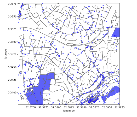
pois[present_keys]

This gives us the relevant points of interest (part of the map). If we’d like to see the entire street network, we can download the entire graph from the location.

graph = ox.graph_from_bbox(north, south, east, west)

# Retrieve nodes and edges
nodes, edges = ox.graph_to_gdfs(graph)

# Get place boundary related to the place name as a geodataframe
area = ox.geocode_to_gdf(place_name)

Which we can then render as follows.

Figure: Points of Interest as identified in Open Street Map.

tourist_places = pois[pois.tourism.notnull()]

Figure: Tourist sites identified as Points of Interest in Open Street Map.

We have the POIs that are associated with tourist places in a geodataframe. To work with them in a machine learning algorithm, it will be easier to conveert them to a pandas DataFrame. This means dealing with the geometry. If we examine the POIs.

tourist_places.loc["node"]

for i in tourist_places["geometry"]["way"]:
    print("latitude: {latitude}, longitude: {longitude}".format(latitude=i.centroid.y, longitude=i.centroid.x))

Matching OpenStreetMap and NMIS Data

In this exercise you will download the location of health centres from OpenStreetMap in Lagos and map them to the health centres you’ve already viewed in the NMIS data. This is a data validation exercise.

Exercise 3

The latitude and longitude of Lagos in Nigeria are as follows:

place_name = "Lagos, Nigeria"

latitude = 6.5244
longitude = 3.3792

In OpenStreetMap the key for a health center is key:healthcare. Download the POIs on OpenStreetMap that are listed as health centres and match them to POIs in the OpenStreetMap data to the health centres we find in the Nigerian NMIS data (pods.datasets.nigeria_nmis).

You may use the distance between the centroid for the match, but you should also consider any additional checks you might wish to perform.

Ensure your code is reusable, making it easy to integrate any necessary human feedback as required.

You may need to vary the size of the bounding box to get matches. Use your reusable code to ensure that you obtain at least five matches between the data set (by increasing bounding box size).

Now further demonstrate the reuse by performing the same analysis for Abuja.

place_name = "Abuja, Nigeria"

latitude = 9.05785 
longitude = 7.49508

Thanks!

For more information on these subjects and more you might want to check the following resources.

• twitter: @lawrennd
• podcast: The Talking Machines
• newspaper: Guardian Profile Page
• blog: http://inverseprobability.com

References