Abstract

In this lab session we look at setting up a SQL server and making joins between different data sets.

Check Session for this Practical is 2nd November 2023

• This practical should prepare you for Part 1 of the course assessment. Ensure that you have a solid understanding of the material, with particular emphasis on the AWS database setup. You should be able to use the same database that you set up here for the final assessment.
• In that assessment, you will be working with significantly larger datasets, often requiring extended waiting times for query execution. Start your work on Part 1 setup early to avoid being blocked from work on subsequent stages later on.
• Some tasks will require you to develop skills for searching for multiple solutions and experimenting with different approaches, which may not have been covered in the lectures. This environment closely resembles real-world data science and software engineering challenges, where there might not be a single correct solution.

Imports, Installs, and Downloads

First, we’re going to download some particular python libraries for dealing with geospatial data. We’re dowloading geopandas which will help us deal with ‘shape files’ that give the geographical lay out of Nigeria. We also need pygeos for indexing.

%pip install geopandas

%pip install pygeos

Setup

notutils

This small package is a helper package for various notebook utilities used below.

The software can be installed using

%pip install notutils

from the command prompt where you can access your python installation.

The code is also available on GitHub: https://github.com/lawrennd/notutils

Once notutils is installed, it can be imported in the usual manner.

import notutils

pods

In Sheffield we created a suite of software tools for ‘Open Data Science’. Open data science is an approach to sharing code, models and data that should make it easier for companies, health professionals and scientists to gain access to data science techniques.

You can also check this blog post on Open Data Science.

The software can be installed using

%pip install pods

from the command prompt where you can access your python installation.

The code is also available on GitHub: https://github.com/lawrennd/ods

Once pods is installed, it can be imported in the usual manner.

import pods

mlai

The mlai software is a suite of helper functions for teaching and demonstrating machine learning algorithms. It was first used in the Machine Learning and Adaptive Intelligence course in Sheffield in 2013.

The software can be installed using

%pip install mlai

from the command prompt where you can access your python installation.

The code is also available on GitHub: https://github.com/lawrennd/mlai

Once mlai is installed, it can be imported in the usual manner.

import mlai

Nigerian Health Facility Distribution

In this notebook, we explore the question of health facility distribution in Nigeria, spatially, and in relation to population density.

We explore and visualize the question “How does the number of health facilities per capita vary across Nigeria?”

Rather than focussing purely on using tools like pandas to manipulate the data, our focus will be on introducing some concepts from databases.

Machine learning can be summarized as \[ \text{model} + \text{data} \xrightarrow{\text{compute}} \text{prediction} \] and many machine learning courses focus a lot on the model part. But to build a machine learning system in practice, a lot of work must be put into the data part. This notebook gives some pointers on that work and how to think about your machine learning systems design.

Datasets

In this notebook, we download 4 datasets:

• Nigeria NMIS health facility data
• Population data for Administrative Zone 1 (states) areas in Nigeria
• Map boundaries for Nigerian states (for plotting and binning)
• Covid cases across Nigeria (as of May 20, 2020)

But joining these data sets together is just an example. As another example, you could think of SafeBoda, a ride-hailing app that’s available in Lagos and Kampala. As well as looking at the health examples, try to imagine how SafeBoda may have had to design their systems to be scalable and reliable for storing and sharing data.

Nigeria NMIS Data

As an example data set we will use Nigerian Millennium Development Goals Information System Health Facility (The Office of the Senior Special Assistant to the President on the Millennium Development Goals (OSSAP-MDGs) and Columbia University, 2014). It can be found here https://energydata.info/dataset/nigeria-nmis-education-facility-data-2014.

Taking from the information on the site,

The Nigeria MDG (Millennium Development Goals) Information System – NMIS health facility data is collected by the Office of the Senior Special Assistant to the President on the Millennium Development Goals (OSSAP-MDGs) in partner with the Sustainable Engineering Lab at Columbia University. A rigorous, geo-referenced baseline facility inventory across Nigeria is created spanning from 2009 to 2011 with an additional survey effort to increase coverage in 2014, to build Nigeria’s first nation-wide inventory of health facility. The database includes 34,139 health facilities info in Nigeria.

The goal of this database is to make the data collected available to planners, government officials, and the public, to be used to make strategic decisions for planning relevant interventions.

For data inquiry, please contact Ms. Funlola Osinupebi, Performance Monitoring & Communications, Advisory Power Team, Office of the Vice President at funlola.osinupebi@aptovp.org

To learn more, please visit http://csd.columbia.edu/2014/03/10/the-nigeria-mdg-information-system-nmis-takes-open-data-further/

Suggested citation: Nigeria NMIS facility database (2014), the Office of the Senior Special Assistant to the President on the Millennium Development Goals (OSSAP-MDGs) & Columbia University

For ease of use we’ve packaged this data set in the pods library

data = pods.datasets.nigeria_nmis()['Y']
data.head()

Alternatively, you can access the data directly with the following commands.

import urllib.request
urllib.request.urlretrieve('https://energydata.info/dataset/f85d1796-e7f2-4630-be84-79420174e3bd/resource/6e640a13-cab4-457b-b9e6-0336051bac27/download/healthmopupandbaselinenmisfacility.csv', 'healthmopupandbaselinenmisfacility.csv')

import pandas as pd
data = pd.read_csv('healthmopupandbaselinenmisfacility.csv')

Once it is loaded in the data can be summarized using the describe method in pandas.

data.describe()

We can also find out the dimensions of the dataset using the shape property.

data.shape

Dataframes have different functions that you can use to explore and understand your data. In python and the Jupyter notebook it is possible to see a list of all possible functions and attributes by typing the name of the object followed by .<Tab> for example in the above case if we type data.<Tab> it show the columns available (these are attributes in pandas dataframes) such as num_nurses_fulltime, and also functions, such as .describe().

For functions we can also see the documentation about the function by following the name with a question mark. This will open a box with documentation at the bottom which can be closed with the x button.

data.describe?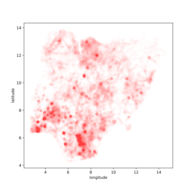

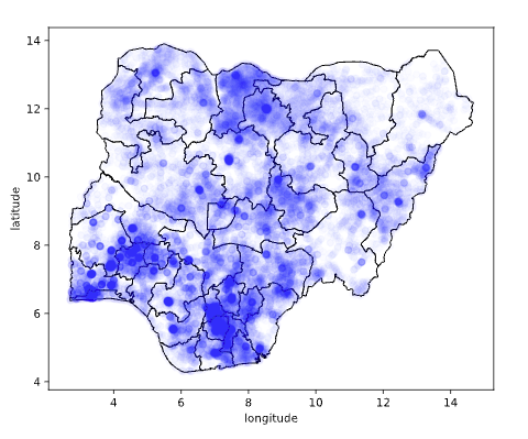
Figure: Location of the over thirty-four thousand health facilities registered in the NMIS data across Nigeria. Each facility plotted according to its latitude and longitude.

hospital_data = data

The upsurge of LLMs is creating opportunities and novel applications in different domains and data science is not the exception. In this section, we want you to explore how LLMs can be included in your data analytics pipelines. Through small examples, we expect to spark your interest in these tools.

We will start by asking questions to an LLM about the nature of our data. We will try to reproduce a data exploration process similar to the one we implemented in the previous section (i.e., data description and visualisation). Before asking questions, we should install the libraries that enable the interaction with LLMs from Python code.

openai Software

The openai library provides an interface for using the OpenAI API from Python applications. You can find more information in its GitHub Repository.

The software can be installed using

%pip install openai

from the command prompt where you can access your python installation.

Once openai is installed, it can be imported in the usual manner.

import openai

Langchain Software

Langchain is a framework to build applications based on LLMs. This library provides functionalities that facilitate the interaction with the models.

The software can be installed using

%pip install langchain

from the command prompt where you can access your python installation.

Once langchain is installed, it can be imported in the usual manner.

import langchain

Langchain agent

Now we should configure a Langchain agent. This agent is the interface between our code and the LLM. The agent receives our questions in natural language and will provide, hopefully, the answer we are looking for.

First let’s import the required libraries.

import os
import pandas as pd
import matplotlib.pyplot as plt
import seaborn as sns
from getpass import getpass
import openai
from langchain.agents import create_pandas_dataframe_agent
from langchain.llms import OpenAI

We need to create an agent using our OpenAI API key now. The agent receives the data we want to analyse as a parameter. In this case, it is the data frame. The verbosity is set to True to track the workflow the agent follows to get the required answer.

openai_api_key = [INSERT_YOUR_OPENAI_API_HERE]
os.environ["OPENAI_API_KEY"] = openai_api_key
openai.api_key = openai_api_key

agent = create_pandas_dataframe_agent(OpenAI(temperature=0, openai_api_key=openai_api_key), data, verbose=True)

Once the agent is configured we can start by asking questions about our data. For example, we can ask the agent for the names of the columns of the dataframe.

results = agent("What are Column names?")

If you look at the output closer, you will see in green the “thoughts” and “actions” the agent performs. It is of particular interest the second “action” of this agent execution chain. This “action” corresponds to the execution ot the df.columns command, where df is the dataframe the agent received as a parameter during its configuration (i.e., the data dataframe). You should get a similar output to the Observation in blue if you execute the data.columns Python command.

data.columns

Let’s go a bit deeper in our analysis. We want to know which columns in our data frame are categorical and which columns store numeric values. Let’s see what the agent says …

results = agent("Which columns are categorical and which are numeric?")

Exercise 1

What is the main command the agent executes to get the answer according to its “actions” and “observations”? Write and execute the Python command using the data data frame in the next box. Compare the output of this execution with the output of the agent “observation”.

In a final example to describe our data, we want to know if there are any missing values in our data frame.

results = agent("Are there any missing values in columns")

Exercise 2

Again, please identify the main command the agend executed and compare the output you get.

The last steps were useful to know the data better. It looks like the integration of LLMs in the process was useful. But, what about data visualisation?

Well, there are already specific libraries designed to this end. That is the case of autoplotlib, which generates plots of your data from text descriptions.

%pip install autoplotlib

Now we can use the library. Let’s ask for a plot of the Nigerian health facilities. The autoplotlib plot function receives the figure description and the data we want to visualise as parameters. The function returns the code of the plot, the figure, and the response from the LLM. These outputs are then prompted to you for checking.

Exercise 3

One nice property of autoplotlib is that it prompts the code before execution. So, you can inspect the code the LLM generates. What do you think of the plotted map? Is it similar to the one we created before?

Certainly, it is similar, but there are some differences. You can add more details to the figure description to make it more similar or change the plot’s appearance. For example, we can change the value of the parameter alpha for the figure. This parameter changes the transparency of the graph, so we can see the places with more density of healthcare facilities.

Now, you have initial ideas about integrating LLMs into the data science process. We will come back to this later in this lab and we expect you to continue thinking of and exploring its potential. For now, let’s save our data frame in a more self-descriptive variable for later. In our next section, we will start learning about Databases.

Databases and Joins

The main idea we will be working with in this practical is the ‘join’. A join does exactly what it sounds like, it combines two database tables.

You may have already started to look at data structures and learning about pandas which is a great way of storing and structuring your data set to make it easier to plot and manipulate your data.

Pandas is great for the data scientist to analyze data because it makes many operations easier. But it is not so good for building the machine learning system. In a machine learning system, you may have to handle a lot of data. Even if you start with building a system where you only have a few customers, perhaps you build an online taxi system (like SafeBoda) for Kampala. Maybe you will have 50 customers. Then maybe your system can be handled with some python scripts and pandas.

Scaling ML Systems

But what if you are successful? What if everyone in Kampala wants to use your system? There are 1.5 million people in Kampala and maybe 100,000 Boda Boda drivers.¹

What if you are even more succesful? What if everyone in Lagos wants to use your system? There are around 20 million people in Lagos … and maybe as many Okada[^okada] drivers as people in Kampala!

[^okada] In Lagos the Boda Boda is called an Okada.

We want to build safe and reliable machine learning systems. Building them from pandas and python is about as safe and reliable as taking six children to school on a boda boda.

To build a reliable system, we need to turn to databases. In this notebook we’ll be focusing on SQL databases and how you bring together different streams of data in a Machine Learning System.

In a machine learning system, you will need to bring different data sets together. In database terminology this is known as a ‘join’. You have two different data sets, and you want to join them together. Just like you can join two pieces of metal using a welder, or two pieces of wood with screws.

But instead of using a welder or screws to join data, we join it using columns of the data. We can join data together using people’s names. One database may contain where people live, another database may contain where they go to school. If we join these two databases, we can have a database which shows where people live and where they got to school.

In the notebook, we will join some data about where the health centers are in Nigeria with data about where there have been cases of Covid19. There are other challenges in the ML System Design that are not going to be covered here. They include how to update the databases and how to control access to the databases from different users (boda boda drivers, riders, administrators etc).

Administrative Zone Geo Data

A very common operation is the need to map from locations in a country to the administrative regions. If we were building a ride sharing app, we might also want to map riders to locations in the city, so that we could know how many riders we had in different city areas.

Administrative regions have various names like cities, counties, districts, or states. These conversions for the administrative regions are important for getting the right information to the right people.

Of course, if we had a knowledgeable Nigerian, we could ask her about what the right location for each of these health facilities is, which state is it in? But given that we have the latitude and longitude, we should be able to find out automatically what the different states are.

This is where “geo” data becomes important. We need to download a dataset that stores the location of the different states in Nigeria. These files are known as ‘outline’ files. Because they draw the different states of different countries in outline.

There are special databases for storing this type of information, the database we are using is in the gdb or GeoDataBase format. It comes in a zip file. Let’s download the outline files for the Nigerian states. They have been made available by the Humanitarian Data Exchange, you can also find other states data from the same site.

Nigerian Administrative Zones Data

For ease of use we’ve packaged this data set in the pods library

data = pods.datasets.nigerian_administrative_zones()['Y']
data.set_index("admin1Name_en", inplace=True)
data.head()

Alternatively you can access the data directly with the following commands.

import zipfile

admin_zones_url = 'https://data.humdata.org/dataset/81ac1d38-f603-4a98-804d-325c658599a3/resource/0bc2f7bb-9ff6-40db-a569-1989b8ffd3bc/download/nga_admbnda_osgof_eha_itos.gdb.zip'
_, msg = urllib.request.urlretrieve(admin_zones_url, 'nga_admbnda_osgof_eha_itos.gdb.zip')
with zipfile.ZipFile('/content/nga_admbnda_osgof_eha_itos.gdb.zip', 'r') as zip_ref:
    zip_ref.extractall('/content/nga_admbnda_osgof_eha_itos.gdb')

import geopandas as gpd
import fiona

states_file = "./nga_admbnda_osgof_eha_itos.gdb/nga_admbnda_osgof_eha_itos.gdb/nga_admbnda_osgof_eha_itos.gdb/nga_admbnda_osgof_eha_itos.gdb/"

layers = fiona.listlayers(states_file)
data = gpd.read_file(states_file, layer=1)
data.crs = "EPSG:4326"
data = data.set_index('admin1Name_en')
    

Figure: Border locations for the thirty-six different states of Nigeria.

zones_gdf = data
zones_gdf['admin1Name_en'] = zones_gdf.index

Now we have this data of the outlines of the different states in Nigeria.

The next thing we need to know is how these health facilities map onto different states in Nigeria. Without “binning” facilities somehow, it’s difficult to effectively see how they are distributed across the country.

We do this by finding a “geo” dataset that contains the spatial outlay of Nigerian states by latitude/longitude coordinates. The dataset we use is of the “gdb” (GeoDataBase) type and comes as a zip file. We don’t need to worry much about this datatype for this notebook, only noting that geopandas knows how to load in the dataset, and that it contains different “layers” for the same map. In this case, each layer is a different degree of granularity of the political boundaries, with layer 0 being the whole country, 1 is by state, or 2 is by local government. We’ll go with a state level view for simplicity, but as an excercise you can change it to layer 2 to view the distribution by local government.

Once we have these MultiPolygon objects that define the boundaries of different states, we can perform a spatial join (sjoin) from the coordinates of individual health facilities (which we already converted to the appropriate Point type when moving the health data to a GeoDataFrame.)

Joining a GeoDataFrame

The first database join we’re going to do is a special one, it’s a ‘spatial join’. We’re going to join the locations of the hospitals with their states.

This join is unusual because it requires some mathematics to get right. The outline files give us the borders of the different states in latitude and longitude, the health facilities have given locations in the country.

A spatial join involves finding out which state each health facility belongs to. Fortunately, the mathematics you need is already programmed for you in GeoPandas. That means all we need to do is convert our pandas dataframe of health facilities into a GeoDataFrame which allows us to do the spatial join.

First, we convert the hospital data to a geopandas data frame.

import geopandas as gpd

geometry = gpd.points_from_xy(hospital_data.longitude, hospital_data.latitude)
hosp_gdf = gpd.GeoDataFrame(hospital_data, 
                            geometry=geometry)
hosp_gdf.crs = "EPSG:4326"

There are some technial details here: the crs refers to the coordinate system in use by a particular GeoDataFrame. EPSG:4326 is the standard coordinate system of latitude/longitude.

Your First Join: Converting GPS Coordinates to States

Now we have the data in the GeoPandas format, we can start converting into states. We will use the fiona library for reading the right layers from the files. Before we do the join, lets plot the location of health centers and states on the same map.

world_gdf = gpd.read_file(gpd.datasets.get_path('naturalearth_lowres'))
world_gdf.crs = "EPSG:4326"
nigeria_gdf = world_gdf[(world_gdf['name'] == 'Nigeria')]

Figure: The outline of the thirty-six different states of nigeria with the location sof the health centers plotted on the map.

Performing the Spatial Join

We’ve now plotted the different health center locations across the states. You can clearly see that each of the dots falls within a different state. For helping the visualization, we’ve made the dots somewhat transparent (we set the alpha in the plot). This means that we can see the regions where there are more health centers, you should be able to spot where the major cities in Nigeria are given the increased number of health centers in those regions.

Of course, we can now see by eye, which of the states each of the health centers belongs to. But we want the computer to do our join for us. GeoPandas provides us with the spatial join. Here we’re going to do a left or outer join.

from geopandas.tools import sjoin

We have two GeoPandas data frames, hosp_gdf and zones_gdf. Let’s have a look at the columns the contain.

hosp_gdf.columns

We can see that this is the GeoDataFrame containing the information about the hospital. Now let’s have a look at the zones_gdf data frame.

zones_gdf.columns

You can see that this data frame has a different set of columns. It has all the different administrative regions. But there is one column name that overlaps. We can find it by looking for the intersection between the two sets.

set(hosp_gdf.columns).intersection(set(zones_gdf.columns))

Here we’ve converted the lists of columns into python ‘sets’, and then looked for the intersection. The join will occur on the intersection between these columns. It will try and match the geometry of the hospitals (their location) to the geometry of the states (their outlines). This match is done in one line in GeoPandas.

We’re having to use GeoPandas because this join is a special one based on geographical locations, if the join was on customer name or some other discrete variable, we could do the join in pandas or directly in SQL.

hosp_state_joined = sjoin(hosp_gdf, zones_gdf, how='left')

The intersection of the two data frames indicates how the two data frames will be joined (if there’s no intersection, they can’t be joined). It’s like indicating the two holes that would need to be bolted together on two pieces of metal. If the holes don’t match, the join can’t be done. There has to be an intersection.

But what will the result look like? Well, the join should be the ‘union’ of the two data frames. We can have a look at what the union should be by (again) converting the columns to sets.

set(hosp_gdf.columns).union(set(zones_gdf.columns))

That gives a list of all the columns (notice that ‘geometry’ only appears once).

Let’s check that’s what the join command did, by looking at the columns of our new data frame, hosp_state_joined. Notice also that there’s a new column: index_right. The two original data bases had separate indices. The index_right column represents the index from the zones_gdf, which is the Nigerian state.

set(hosp_state_joined.columns)

Great! They are all there! We have completed our join. We had two separate data frames with information about states and information about hospitals. But by performing an ‘outer’ or a ‘left’ join, we now have a single data frame with all the information in the same place! Let’s have a look at the first frew entries in the new data frame.

hosp_state_joined.head()

SQL Database

Our first join was a special one, because it involved spatial data. That meant using the special gdb format and the GeoPandas tool for manipulating that data. But we’ve now saved our updated data in a new file.

To do this, we use the command line utility that comes standard for SQLite database creation. SQLite is a simple database that’s useful for playing with database commands on your local machine. For a real system, you would need to set up a server to run the database. The server is a separate machine with the job of answering database queries. SQLite pretends to be a proper database but doesn’t require us to go to the extra work of setting up a server. Popular SQL server software includes MariaDB which is open source, or Microsoft’s SQL Server.

A typical machine learning installation might have you running a database from a cloud service (such as AWS, Azure or Google Cloud Platform). That cloud service would host the database for you, and you would pay according to the number of queries made.

Many start-up companies were formed on the back of a MySQL server hosted on top of AWS. Although since MySQL was sold to Sun, and then passed on to Oracle, the open source community has turned its attention to MariaDB, here’s the AWS instructions on how to set up MariaDB.

If you were designing your own ride hailing app, or any other major commercial software you would want to investigate whether you would need to set up a central SQL server in one of these frameworks.

Create the MariaDB Instance

hosp_state_joined.to_csv('hospitals_zones_joined.csv', header=None)

We will now set up a MariaDB database instance for storing our data.

Creating a MariaDB Server on AWS

In this section we’ll go through the set up required to create a MariaDB server on AWS.

Before you start, you’re going to need a username and password for accessing the database. You will need to tell the MariaDB server what that username and password is, and you’ll also need to make use of it when your client connects to the database. It’s good practice to never expose passwords in your code directly. So to protect your passowrd, we’re going to create a credentials.yaml file locally that will store your username and password so that the client can access the server without ever showing your password in the notebook.

We suggest you set the username as admin and make secure choice of password for your password.

We’ll use the following code for recording the username and password for the SQL client.

Saving a Credentials File

import yaml
from ipywidgets import interact_manual, Text, Password

If you click Run Interact then the credentials you’ve selected will be saved in the yaml file. Remember them, as you’ll need them when you set up the database server below.

Brief History of the Cloud

In the early days of the internet, companies could make use of open source software, such as the Apache web server and the MySQL database for providing on line stores, or other capabilities. But as part of that, they normally had to provide their own server farms. For example, the earliest server for running PageRank from 1996 was hosted on custom made hardware built in a case of Mega Blocks (see Figure \(\ref{the-first-google-computer-at-stanford}\)).

Figure: The web search engine was hosted on custom built hardware. Photo credit Christian Heilmann on Flickr.

By September 2000, Google operated 5000 PCs for searching and web crawling, using the LINUX operating system.²

Cloud computing gives you access to computing at a similar scale, but on an as-needed basis. AWS launched S3 cloud storage in March 2006 and the Elastic Compute Cloud followed in August 2006. These services were inspired by the challenges they had scaling their own web service (known as Obidos) for running the world’s largest e-commerce site. Recent market share estimates indicate that AWS still retains around a third of the cloud infrastructure market.³

The earliest AWS services of S3 and EC2 gave storage and compute. Together these could be combined to host a database service. Today cloud providers also provide machines that are already set up to provide a database service. We will make use of AWS’s Relational Database Service to provide our MariaDB server.

1. Log in to your AWS account and go to the AWS RDS console here.

2. Make sure the region is set to Europe (London) which is denoted as eu-west-2.

3. Scroll down to “Create Database”. Do not create an Aurora database instance.

4. Standard Create should be selected. In the box below, which is titled Engine Options you should select MariaDB. You can leave the Version as it’s set,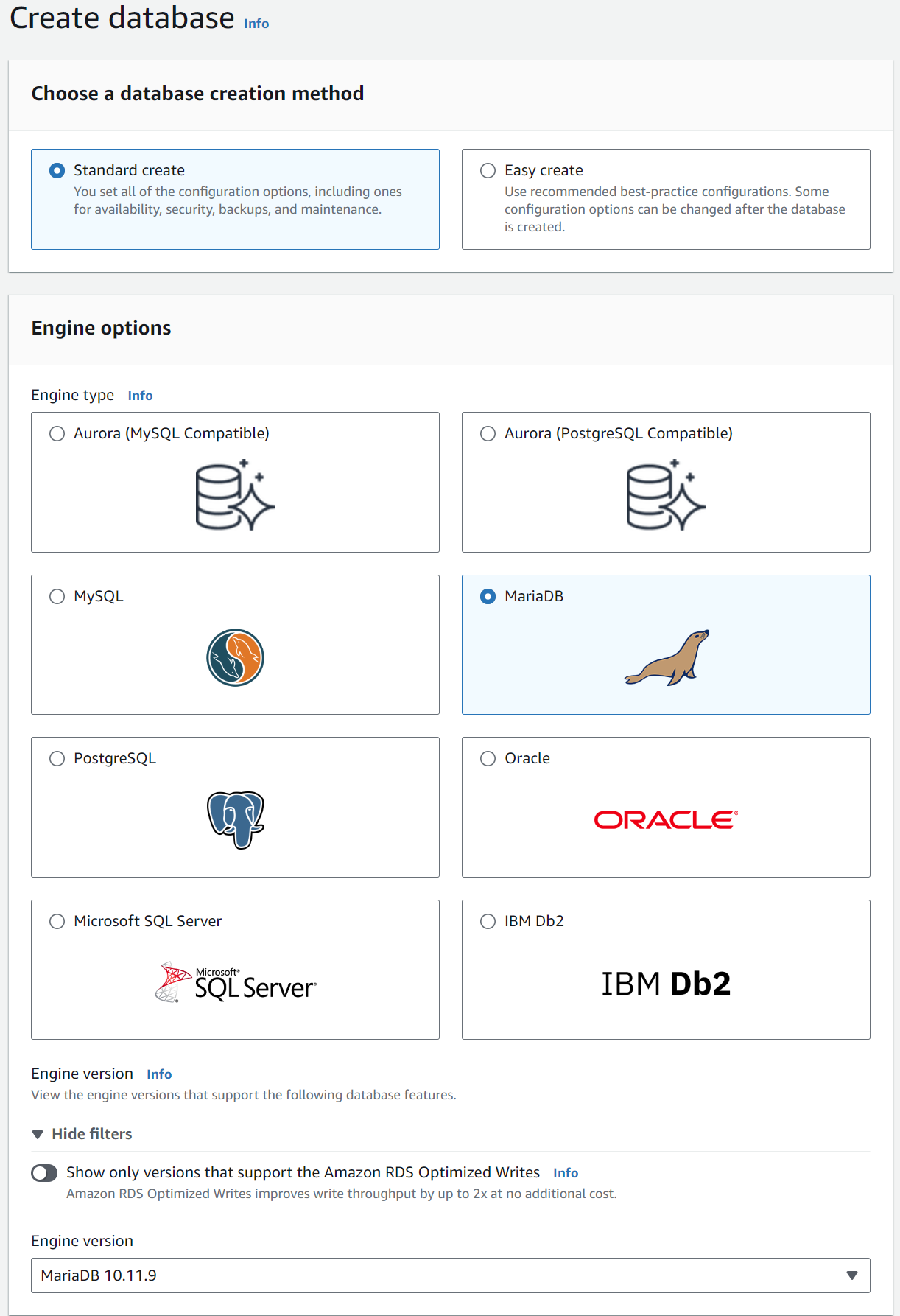

   

   

   Figure: The AWS console box for selecting the MariaDB database.

5. In the box below that, make sure you select Free tier.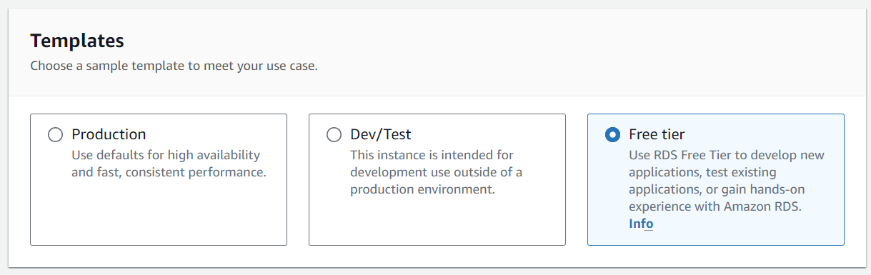

   

   

   Figure: Make sure you select the free tier option for your database.

6. Name your database. For this setup we suggest you use testdatabase-mariadb for the name.

7. Set a master password for accessing the data base as admin.

   

   

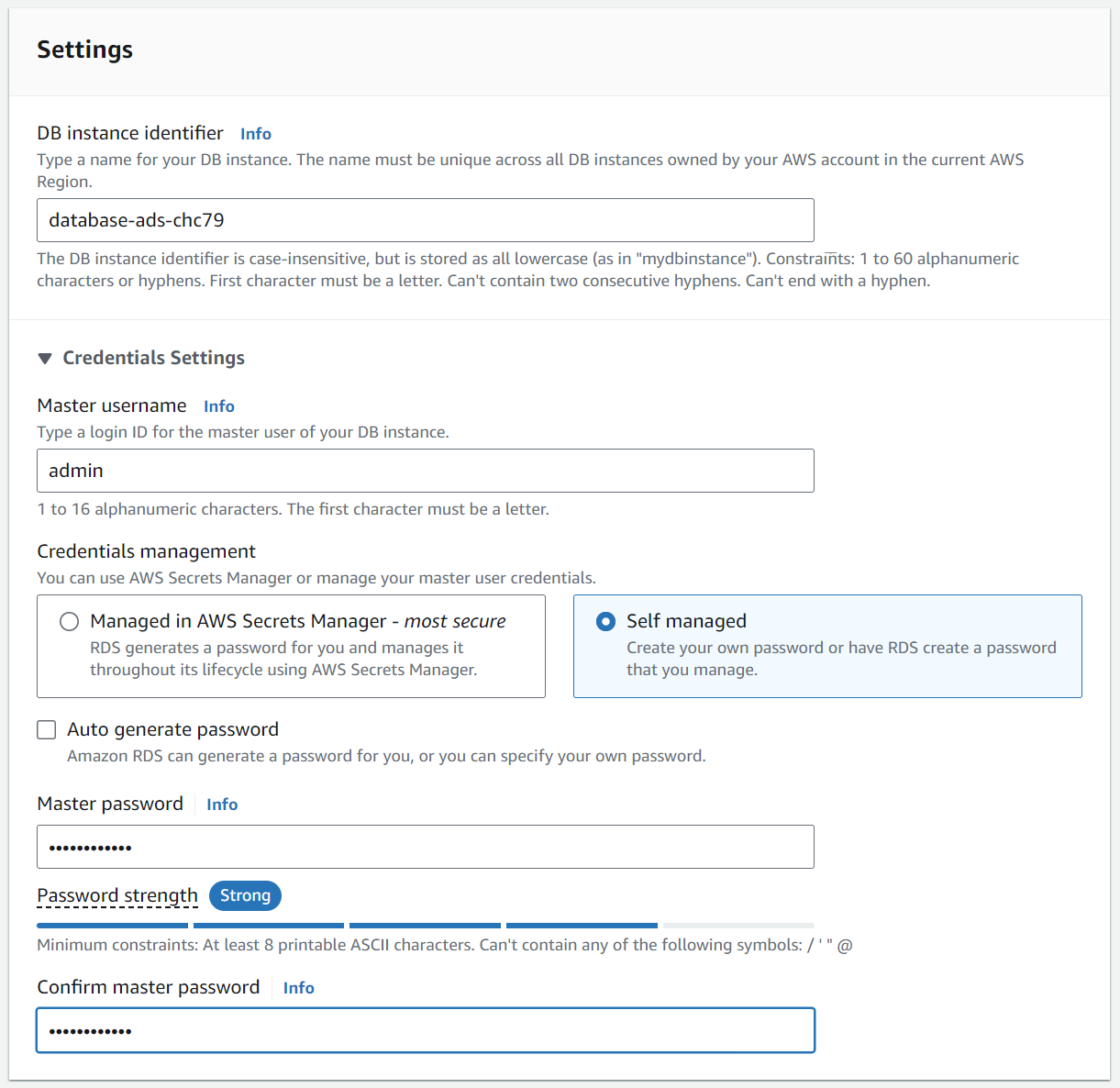
   Figure: Set the password and username for the database access.

8. Leave the DB instance class as it is.

9. Leave the DB instance size at the default setting. Leave the storage type and allocated storage at the default settings of General Purpose (SSD) and 20.

10. Disable autoscaling.

11. In the connectivity leave VPC selection as Default VPC and enable Publicly accessible so that you’ll have an IP address for your database.

12. In VPC security group select Create new to create a new security group for the instance.

13. Write ADSMariaDB as the group name for the VPC security group.

14. Select Create database at the bottom to launch the database.}

Your database will take a few minutes to launch.

While it’s launching you can check the access rules for the database here.

1. Select the Default security group.
2. The source of the active inbound rule must be set to 0.0.0.0/0. It means you can connect from any source using IPv4.

A wrong inbound rule can cause you fail connecting to the database from this notebook.

Note: by setting the inbound rule to 0.0.0.0/0 we have opened up access to any IP address. If this were production code you wouldn’t do this, you would specify a range of addresses or the specific address of the compute server that needed to access the system. Because we’re using Google colab or another notebook client to access, and we can’t control the IP address of that access, for simplicity we’ve set it up so that any IP address can access the database, but that is not good practice for production systems.

Once the database is up and running you should be able to find its url on this page. You can add that to the credentials file using the following code.

# Insert your database url below
database_details = {"url": INSERT_YOUR_DATABASE_URL_HERE, 
                    "port": 3306}

%pip install ipython-sql

%pip install PyMySQL

%load_ext sql

with open("credentials.yaml") as file:
  credentials = yaml.safe_load(file)
username = credentials["username"]
password = credentials["password"]
url = database_details["url"]

Connect to the database, enabling the uploading of local files as part of the connection.

%sql mariadb+pymysql://$username:$password@$url?local_infile=1

Now that we have the database connection, we’re going to create a new database called nigeria_nmis for doing our work in.

%%sql
SET SQL_MODE = "NO_AUTO_VALUE_ON_ZERO";
SET time_zone = "+00:00";

CREATE DATABASE IF NOT EXISTS `nigeria_nmis` DEFAULT CHARACTER SET utf8 COLLATE utf8_bin;

%%sql
USE `nigeria_nmis`;

For the data to be loaded in to the table, we need to describe the schema. The schema tells the database server what to expect in the columns of the table.

%%sql
--
-- Table structure for table `hospitals_zones_joined`
--
DROP TABLE IF EXISTS `hospitals_zones_joined`;
CREATE TABLE IF NOT EXISTS `hospitals_zones_joined` (
  `db_id` bigint(20) unsigned NOT NULL,
  `facility_name` tinytext COLLATE utf8_bin NOT NULL,
  `facility_type_display` tinytext COLLATE utf8_bin NOT NULL,
  `maternal_health_delivery_services` BOOLEAN COLLATE utf8_bin NOT NULL,
  `emergency_transport` BOOLEAN COLLATE utf8_bin NOT NULL,
  `skilled_birth_attendant` BOOLEAN COLLATE utf8_bin NOT NULL,
  `num_chews_fulltime` bigint(20) unsigned NOT NULL,
  `phcn_electricity` BOOLEAN COLLATE utf8_bin NOT NULL,
  `c_section_yn` BOOLEAN COLLATE utf8_bin NOT NULL,
  `child_health_measles_immun_calc` BOOLEAN COLLATE utf8_bin NOT NULL,
  `num_nurses_fulltime` bigint(20) unsigned NOT NULL,
  `num_nursemidwives_fulltime` bigint(20) unsigned NOT NULL,
  `num_doctors_fulltime` bigint(20) unsigned NOT NULL,
  `date_of_survey` date NOT NULL,
  `facility_id` tinytext COLLATE utf8_bin NOT NULL,
  `community` tinytext COLLATE utf8_bin NOT NULL,
  `ward` tinytext COLLATE utf8_bin NOT NULL,
  `management` tinytext COLLATE utf8_bin NOT NULL,
  `improved_water_supply` BOOLEAN COLLATE utf8_bin NOT NULL,
  `improved_sanitation` BOOLEAN COLLATE utf8_bin NOT NULL,
  `vaccines_fridge_freezer` BOOLEAN COLLATE utf8_bin NOT NULL,
  `antenatal_care_yn` BOOLEAN COLLATE utf8_bin NOT NULL,
  `family_planning_yn` BOOLEAN COLLATE utf8_bin NOT NULL,
  `malaria_treatment_artemisinin` BOOLEAN COLLATE utf8_bin NOT NULL,
  `sector` tinytext COLLATE utf8_bin NOT NULL,
  `formhub_photo_id` tinytext COLLATE utf8_bin NOT NULL,
  `gps` tinytext COLLATE utf8_bin NOT NULL,
  `survey_id` tinytext COLLATE utf8_bin NOT NULL,
  `unique_lga` tinytext COLLATE utf8_bin NOT NULL,
  `latitude` decimal(11,8) NOT NULL,
  `longitude` decimal(10,8) NOT NULL,
  `geometry` tinytext COLLATE utf8_bin NOT NULL,
  `index_right` bigint(20) unsigned NOT NULL,
  `admin1Name_en` tinytext COLLATE utf8_bin NOT NULL,
  `admin1Pcode` tinytext COLLATE utf8_bin NOT NULL,
  `admin1RefName` tinytext COLLATE utf8_bin NOT NULL,
  `admin1AltName1_en` tinytext COLLATE utf8_bin NOT NULL,
  `admin1AltName2_en` tinytext COLLATE utf8_bin NOT NULL,
  `admin0Name_en` tinytext COLLATE utf8_bin NOT NULL,
  `admin0Pcode` tinytext COLLATE utf8_bin NOT NULL,
  `date` date NOT NULL,
  `validOn` date NOT NULL,
  `validTo` date NOT NULL,
  `Shape_Length` decimal(10,10) NOT NULL,
  `Shape_Area` decimal(10,10) NOT NULL  
) DEFAULT CHARSET=utf8 COLLATE=utf8_bin AUTO_INCREMENT=1 ;

We also need to tell the server what the index of the data base is. Here we’re adding db_id as the primary key in the index.

%%sql
--
-- Indexes for table `hospitals_zones_joined`
--
ALTER TABLE `hospitals_zones_joined`
 ADD PRIMARY KEY (`db_id`);

%%sql
--
-- AUTO_INCREMENT for table `hospitals_zones_joined`
--
ALTER TABLE `hospitals_zones_joined`
MODIFY `db_id` bigint(20) unsigned NOT NULL AUTO_INCREMENT,AUTO_INCREMENT=1;

Now we’re ready to load the data into the table. This can be done with the SQL command LOAD DATA. When connecting to the database we used the flag local_infile=1 to ensure we could load local files into the database.

%%sql
LOAD DATA LOCAL INFILE 'hospitals_zones_joined.csv' INTO TABLE hospitals_zones_joined
FIELDS TERMINATED BY ','
LINES STARTING BY '' TERMINATED BY '\n';

%sql SELECT * FROM hospitals_zones_joined LIMIT 10

In the database there can be several ‘tables’. Each table can be thought of as like a separate dataframe. The table name we’ve just saved is hospitals_zones_joined.

Accessing the SQL Database

Now that we have a SQL database, we can create a connection to it and query it using SQL commands. Let’s try to simply select the data we wrote to it, to make sure it’s the same.

Start by making a connection to the database. This will often be done via remote connections, but for this example we’ll connect locally to the database using the filepath directly.

To access a data base, the first thing that is made is a connection. Then SQL is used to extract the information required. A typical SQL command is SELECT. It allows us to extract rows from a given table. It operates a bit like the .head() method in pandas, it will return the first N rows (by default the .head() command returns the first 5 rows, but you can set N to whatever you like. Here we’ve included a default value of 5 to make it match the pandas command.

We do this using an execute command on the connection.

Typically, its good software engineering practice to ‘wrap’ the database command in some python code. This allows the commands to be maintained. You will also be asked to do this in your final assessment, including re-writing some of the code - pay attention to the slight syntax differences and multi-statement queries.Below we wrap the SQL command

SELECT * FROM table_name LIMIT N

in python code. This SQL command selects the first N entries from a given database called table_name.

We can pass the table_name and number of rows, n, to the python command.

Now we make the connection using the details stored in credentials and database_details.

conn = create_connection(user=credentials["username"], 
                         password=credentials["password"], 
                         host=database_details["url"],
                         database="nigeria_nmis")

Now that we have a connection, we can write a command and pass it to the database.

The python library, pymysql, allows us to access the SQL database directly from python.

Let’s have a go at calling the command to extract the first three facilities from our health center database. Let’s try creating a function that does the same thing the pandas .head() method does so we can inspect our database.

def head(conn, table, n=5):
  rows = select_top(conn, table, n)
  for r in rows:
      print(r)

head(conn, "hospitals_zones_joined")

Great! We now have the database in and some python functions that operate on the data base by wrapping SQL commands.

We will return to the SQL command style after download and add the other datasets to the database using a combination of pandas and the database utilities.

Our next task will be to introduce data on COVID19 so that we can join that to our other data sets.

Databases and Large Language Models

In a previous section, we integrated LLMs in the data exploration and visualisation process. Now we will see the potential of integrating LLMs for databases. We will use the agend we created before using langchain and describe the instruction we need the agent to execute.

sql_code = agent("The database 'nigeria_nmis' is hosted in AWS the endpoint is '" + url + "'. The user is '" + username + "' and the password '" + password + "'. The database has the table hospitals_zones_joined with columns facility_name and num_nurses_fulltime (number of full time nurses), give pymysql mariadb code to show the 20 hospitals which have the most full time nurses. Print the results of the query as a dataframe at the end")

If you analyse the input that the agent receives, we need to be more specific this time. We passed the name of the database we wanted to use, the AWS endpoint, the username, and the password of our database. Then we provide information about the table we want to query (e.g., table name and columns). Finally, we provide the data requirement we need to satisfy (i.e., show the 20 hospitals which have the most full time nurses), and specify how these should be printed.

Similarly, the “actions” and “observations are a bit more complex compared to the output of previous data exploration tasks.

For comparison, we can execute the SQL command that the model generates directly in our database.

%sql SELECT facility_name, num_nurses_fulltime FROM hospitals_zones_joined ORDER BY num_nurses_fulltime DESC LIMIT 20

As the interaction with the LLM becomes more and more complex, it is a good idea to think about code wrappers that we can reuse in our pipeline. For example, we can define a set of Python functions that facilitate the database and LLMs integration. A way to define these functions, but not the only one, is presented as follows:

def simple_llm_sql(command, dbname='nigeria_nmis', tables=('hospitals_zones_joined',)):
    sql_code = llm_prompt(f"In this database '{dbname}' with: " + ", ".join([f"table {table} described {sql_query(f'DESCRIBE {table}')}" for table in tables]) + f", give pymysql mariadb code to: {command}. Format your response as only the SQL query, not python code, not description.") # experiment with prompts
    print(sql_code)
    y = input('safe to execute? (y/n)')
    if y == 'y':
      return sql_query(sql_code)

def sql_query(query, host='database-ads.cgrre17yxw11.eu-west-2.rds.amazonaws.com', user=username, password=password, db='nigeria_nmis'):
  conn = create_connection(user, password, host, db)
  return pd.read_sql(query, conn)

def llm_prompt(llm_prompt, model="gpt-3.5-turbo"):
  return openai.ChatCompletion.create(
      model=model,
      messages = [{"role": "user", "content": llm_prompt}],
      temperature=0.2,
      max_tokens=2000,
      frequency_penalty=0.0
  ).choices[0].message.content

Then, we can call our wrapper in a simplified fashion.

simple_llm_sql("show the 20 hospitals which have the most full time nurses")

We will return to the SQL command style after downloading and adding the other datasets to the database using a combination of pandas and the database utilities.

Our next task will be to introduce data on COVID19 so that we can join that to our other data sets.

Covid Data

Now we have the health data, we’re going to combine it with data about COVID-19 cases in Nigeria over time. This data is kindly provided by Africa open COVID-19 data working group, which Elaine Nsoesie has been working with. The data is taken from Twitter, and only goes up until May 2020.

They provide their data in GitHub. We can access the cases we’re interested in from the following URL.

https://raw.githubusercontent.com/dsfsi/covid19africa/master/data/line_lists/line-list-nigeria.csv

For convenience, we’ll load the data into pandas first, but our next step will be to create a new SQLite table containing the data. Then we’ll join that table to our existing tables.

Nigerian COVID Data

At the beginning of the COVID-19 outbreak, the Consortium for African COVID-19 Data formed to bring together data from across the African continent on COVID-19 cases (Marivate et al., 2020). These cases are recorded in the following GitHub repository: https://github.com/dsfsi/covid19africa.

For ease of use we’ve packaged this data set in the pods library

import pods

data = pods.datasets.nigerian_covid()['Y']
data.head()

Alternatively, you can access the data directly with the following commands.

import urllib.request
import pandas as pd

urllib.request.urlretrieve('https://raw.githubusercontent.com/dsfsi/covid19africa/master/data/line_lists/line-list-nigeria.csv', 'line-list-nigeria.csv')
data = pd.read_csv('line-list-nigeria.csv', parse_dates=['date', 
                                                         'date_confirmation', 
                                                         'date_admission_hospital', 
                                                         'date_onset_symptoms',
                                                         'death_date'])

Once it is loaded in the data can be summarized using the describe method in pandas.

data.describe()

Figure: Evolution of COVID-19 cases in Nigeria.

covid_data=data
covid_data.to_csv('cases.csv', header=None)

Now we convert this CSV file we’ve downloaded into a new table in the database file.

Once again we have to construct a schema for the data.

%%sql
--
-- Table structure for table `cases`
--
DROP TABLE IF EXISTS `cases`;
CREATE TABLE IF NOT EXISTS `cases` (
  `index` int(10) unsigned NOT NULL,
  `case_id` int(10) unsigned NOT NULL,
  `origin_case_id` int(10) unsigned NOT NULL,
  `date` date NOT NULL,
  `age` int(10),
  `gender` tinytext COLLATE utf8_bin NOT NULL,
  `city` tinytext COLLATE utf8_bin NOT NULL,
  `province/state` tinytext COLLATE utf8_bin NOT NULL,
  `country` tinytext COLLATE utf8_bin NOT NULL,
  `current_status` tinytext COLLATE utf8_bin,
  `source` text COLLATE utf8_bin,
  `symptoms` text COLLATE utf8_bin,
  `date_onset_symptoms` date,
  `date_admission_hospital` date,
  `date_confirmation` date,
  `underlying_conditions` text COLLATE utf8_bin,
  `travel_history_dates` text COLLATE utf8_bin,
  `travel_history_location` text COLLATE utf8_bin,
  `death_date` date,
  `notes_for_discussion` text COLLATE utf8_bin,
  `Unnamed: 19` text COLLATE utf8_bin
) DEFAULT CHARSET=utf8 COLLATE=utf8_bin AUTO_INCREMENT=1 ;

Once again we need to set the index.

%%sql
--
-- Indexes for table `cases`
--
ALTER TABLE `cases`
 ADD PRIMARY KEY (`index`);

And now we can load the data into the table.

%%sql
LOAD DATA LOCAL INFILE 'cases.csv' INTO TABLE cases
FIELDS TERMINATED BY ','
LINES STARTING BY '' TERMINATED BY '\n';

Population Data

Now we have information about COVID cases, and we have information about how many health centers and how many doctors and nurses there are in each health center. But unless we understand how many people there are in each state, then we cannot make decisions about where they may be problems with the disease.

If we were running our ride hailing service, we would also need information about how many people there were in different areas, so we could understand what the demand for the boda boda rides might be.

To access the number of people we can get population statistics from the Humanitarian Data Exchange.

We also want to have population data for each state in Nigeria, so that we can see attributes like whether there are zones of high health facility density but low population density.

import urllib

pop_url = "https://data.humdata.org/dataset/a7c3de5e-ff27-4746-99cd-05f2ad9b1066/resource/d9fc551a-b5e4-4bed-9d0d-b047b6961817/download/nga_admpop_adm1_2020.csv"
_, msg = urllib.request.urlretrieve(pop_url,"nga_admpop_adm1_2020.csv")
data = pd.read_csv("nga_admpop_adm1_2020.csv")

To do joins with this data, we must first make sure that the columns have the right names. The name should match the same name of the column in our existing data. So we reset the column names, and the name of the index, as follows.

data.dropna(axis=0, how="all", inplace=True)
data.dropna(axis=1, how="all", inplace=True)
data.rename(columns = {"ADM0_NAME" : "admin0Name_en", 
                       "ADM0_PCODE" : "admin0Pcode", 
                       "ADM1_NAME" : "admin1Name_en", 
                       "ADM1_PCODE" : "admin1Pcode", 
                       "T_TL" : "population"},
            inplace=True)
data["admin0Name_en"] = data["admin0Name_en"].str.title()
data["admin1Name_en"] = data["admin1Name_en"].str.title()
    
data = data.set_index("admin1Name_en")

data = pods.datasets.nigerian_population()["Y"]

data.head()

pop_data=data

When doing this for real world data, you should also make sure that the names used in the rows are the same across the different data bases. For example, has someone decided to use an abbreviation for ‘Federal Capital Territory’ and set it as ‘FCT’. The computer won’t understand these are the same states, and if you do a join with such data, you can get duplicate entries or missing entries. This sort of thing happens a lot in real world data and takes a lot of time to sort out. Fortunately, in this case, the data is well curated, and we don’t have these problems.

Save to database file

The next step is to add this new CSV file as an additional table in our database.

Loading the Population Data into the MariaDB

We can load the data into MariaDB using the following sequence of SQL..

pop_data.to_csv('pop_data.csv')

Computing per capita hospitals and COVID

The Minister of Health in Abuja may be interested in which states are most vulnerable to COVID19. We now have all the information in our SQL data bases to compute what our health center provision is per capita, and what the COVID19 situation is.

To do this, we will use the JOIN operation from SQL and introduce a new operation called GROUPBY.

Joining in Pandas

As before, these operations can be done in pandas or GeoPandas. Before we create the SQL commands, we’ll show how you can do that in pandas.

In pandas, the equivalent of a database table is a dataframe. So, the JOIN operation takes two dataframes and joins them based on the key. The key is that special shared column between the two tables. The place where the ‘holes align’ so the two databases can be joined together.

In GeoPandas we used an outer join. In an outer join you keep all rows from both tables, even if there is no match on the key. In an inner join, you only keep the rows if the two tables have a matching key.

This is sometimes where problems can creep in. If in one table Abuja’s state is encoded as ‘FCT’ or ‘FCT-Abuja’, and in another table it’s encoded as ‘Federal Capital Territory’, they won’t match, and that data wouldn’t appear in the joined table.

In simple terms, a JOIN operation takes two tables (or dataframes) and combines them based on some key, in this case the index of the Pandas data frame which is the state name.

zones_gdf.set_index("admin1Name_en", inplace=True)
pop_joined = zones_gdf.join(pop_data['population'], how='inner')

GroupBy in Pandas

Our COVID19 data is in the form of individual cases. But we are interested in total case counts for each state. There is a special data base operation known as GROUP BY for collecting information about the individual states. The type of information you might want could be a sum, the maximum value, an average, the minimum value. We can use a GroupBy operation in pandas and SQL to summarize the counts of covid cases in each state.

A GROUPBY operation groups rows with the same key (in this case ‘province/state’) into separate objects, that we can operate on further such as to count the rows in each group, or to sum or take the mean over the values in some column (imagine each case row had the age of the patient, and you were interested in the mean age of patients.)

covid_cases_by_state = covid_data.groupby(['province/state']).count()['case_id']

The .groupby() method on the dataframe has now given us a new data series that contains the total number of covid cases in each state. We can examine it to check we have something sensible.

covid_cases_by_state

Now we have this new data series, it can be added to the pandas dataframe as a new column.

pop_joined['covid_cases_by_state'] = covid_cases_by_state

The spatial join we did on the original data frame to obtain hosp_state_joined introduced a new column, index_right that contains the state of each of the hospitals. Let’s have a quick look at it below.

hosp_state_joined['index_right']

To count the hospitals in each of the states, we first create a grouped series where we’ve grouped on these states.

grouped = hosp_state_joined.groupby('admin1Name_en')

This python operation now goes through each of the groups and counts how many hospitals there are in each state. It stores the result in a dictionary. If you’re new to python, then to understand this code you need to understand what a ‘dictionary comprehension’ is. In this case the dictionary comprehension is being used to create a python dictionary of states and total hospital counts. That’s then being converted into a pandas Data Series and added to the pop_joined dataframe.

import pandas as pd

counted_groups = {k: len(v) for k, v in grouped.groups.items()}
pop_joined['hosp_state'] = pd.Series(counted_groups)

For convenience, we can now add a new data series to the data frame that contains the per capita information about hospitals. that makes it easy to retrieve later.

pop_joined['hosp_per_capita_10k'] = (pop_joined['hosp_state'] * 10000 )/ pop_joined['population']

SQL-style

That’s the pandas approach to doing it. But pandas itself is inspired by database languages, in particular relational databases such as SQL. To do these types of joins at scale, e.g., for a ride hailing app, we need to do these joins in a database.

As before, we’ll wrap the underlying SQL commands with a convenient python command.

What you see below gives the full SQL command. There is a SELECT command, which extracts FROM a particular table. It then completes an INNER JOIN using particular columns (province/state and admin1Name_en)

Now we’ve created our python wrapper, we can connect to the data base and run our SQL command on the database using the wrapper.

conn = create_connection(user=credentials["username"], 
                         password=credentials["password"],
             host=database_details["url"],
             database="nigeria_nmis")

state_cases_hosps = join_counts(conn)

for row in state_cases_hosps:
    print("State {} \t\t Covid Cases {} \t\t Health Facilities {}".format(row[0], row[1], row[2]))

base = nigeria_gdf.plot(color='white', edgecolor='black', alpha=0, figsize=(11, 11))
pop_joined.plot(ax=base, column='population', edgecolor='black', legend=True)
base.set_title("Population of Nigerian States")

base = nigeria_gdf.plot(color='white', edgecolor='black', alpha=0, figsize=(11, 11))
pop_joined.plot(ax=base, column='hosp_per_capita_10k', edgecolor='black', legend=True)
base.set_title("Hospitals Per Capita (10k) of Nigerian States")

Exercise 4

Add a new column the dataframe for covid cases per 10,000 population, in the same way we computed health facilities per 10k capita.

Exercise 5

Add a new column for covid cases per health facility.

Exercise 6

Do this in both the SQL and the Pandas styles to get a feel for how they differ.

Exercise 7

Perform an inner join using SQL on your databases and convert the result into a pandas DataFrame.

# pop_joined['cases_per_capita_10k'] = ???
# pop_joined['cases_per_facility'] = ???

base = nigeria_gdf.plot(color='white', edgecolor='black', alpha=0, figsize=(11, 11))
pop_joined.plot(ax=base, column='cases_per_capita_10k', edgecolor='black', legend=True)
base.set_title("Covid Cases Per Capita (10k) of Nigerian States")

base = nigeria_gdf.plot(color='white', edgecolor='black', alpha=0, figsize=(11, 11))
pop_joined.plot(ax=base, column='covid_cases_by_state', edgecolor='black', legend=True)
base.set_title("Covid Cases by State")

base = nigeria_gdf.plot(color='white', edgecolor='black', alpha=0, figsize=(11, 11))
pop_joined.plot(ax=base, column='cases_per_facility', edgecolor='black', legend=True)
base.set_title("Covid Cases per Health Facility")

Exercise 8

Interact with LLMs using the tools shown above to describe and visualise an aspect of the dataframe from question 4.

Thanks!

For more information on these subjects and more you might want to check the following resources.

• twitter: @lawrennd
• podcast: The Talking Machines
• newspaper: Guardian Profile Page
• blog: http://inverseprobability.com

References